WHY scaling matrices?

Generally, if you don’t center columns of a matrix before PCA, you end up with the loadings of PC1 being the column means, which is not of must interest.

n <- 100; m <- 10
a <- matrix(0, n, m); a[] <- rnorm(length(a))
a <- sweep(a, 2, 1:m, '+')
colMeans(a)

##  [1]  0.9969826  1.9922219  3.0894905  3.9680835  4.9433477  6.0007352
##  [7]  6.9524794  8.0898546  8.9506657 10.0354630

pca <- prcomp(a, center = FALSE)
cor(pca$rotation[, 1], colMeans(a))

## [1] 0.9999991

Now, say you have centered column or your matrix, do you also need to scale them? That is to say, do they need to have the same norm or standard deviation?

PCA consists in finding an orthogonal basis that maximizes the variation in the data you analyze. So, if there is a column with much more variation than the others, it will probably end up being PC1, which is not of must interest.

n <- 100; m <- 10
a <- matrix(0, n, m); a[] <- rnorm(length(a))
a[, 1] <- 100 * a[, 1]
apply(a, 2, sd)

##  [1] 90.8562836  0.8949268  0.9514208  1.0437561  0.9995103  1.0475651
##  [7]  0.9531466  0.9651383  0.9804789  0.9605121

pca <- prcomp(a, center = TRUE)
pca$rotation[, 1]

##  [1]  9.999939e-01  6.982439e-04 -5.037773e-04 -9.553513e-05  8.937869e-04
##  [6] -1.893732e-03 -3.053232e-04  1.811950e-03 -1.658014e-03  9.937442e-04

Hope I convinced you on WHY it is important to scale matrix columns before doing PCA. I will now show you HOW not to do it explictly.

Reimplementation of PCA

In this part, I will show you the basic code if you want to reimplement PCA yourself. It will serve as a basis to show you how to do linear algebra on a scaled matrix, without explicitly scaling the matrix.

# True one
n <- 100; m <- 10
a <- matrix(0, n, m); a[] <- rnorm(length(a))
pca <- prcomp(a, center = TRUE, scale. = TRUE)
# DIY
a.scaled <- scale(a, center = TRUE, scale = TRUE)
K <- crossprod(a.scaled)
K.eigs <- eigen(K, symmetric = TRUE)
v <- K.eigs$vectors
PCs <- a.scaled %*% v
# Verif, recall that PCs can be opposites between runs
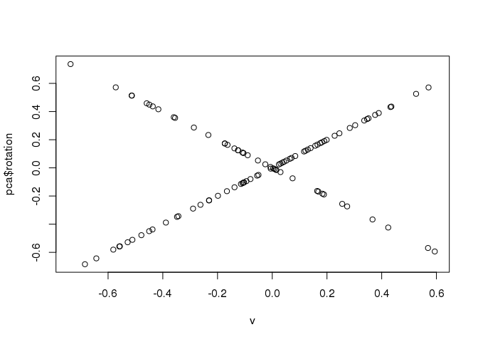
plot(v, pca$rotation)

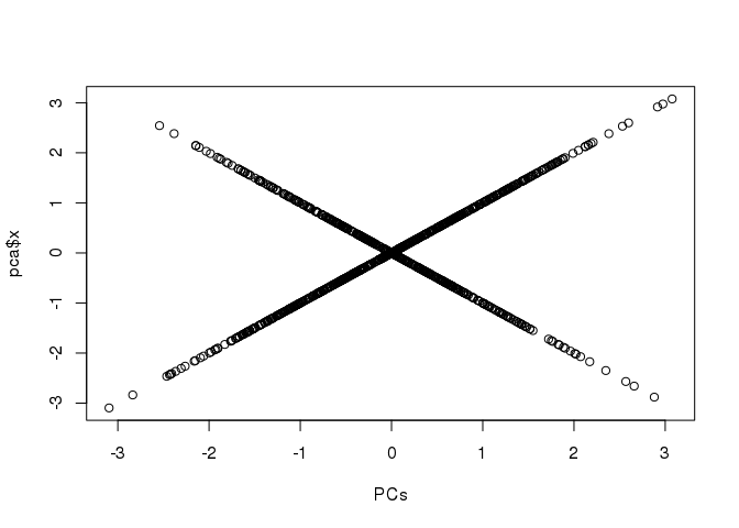
all.equal(sqrt(K.eigs$values), sqrt(n - 1) * pca$sdev)

## [1] TRUE

plot(PCs, pca$x)

Linear algebra behind the previous implementation

Suppose \(m < n\) (\(m\) is the number of columns and \(n\) is the number of rows). Let us denote \(\tilde{X}\) the scaled matrix. A partial singular value decomposition of \(\tilde{X}\) is \(\tilde{X} \approx U \Delta V^T\) where \(U\) is an \(n \times K\) matrix such that \(U^T U = I_K\), \(\Delta\) is a \(K \times K\) diagonal matrix and \(V\) is an \(m \times K\) matrix such that \(V^T V = I_K\). Taking \(K = m\), you end up with \(\tilde{X} = U \Delta V^T\).

\(U \Delta\) are the scores (PCs) of the PCA and \(V\) are the loadings (rotation coefficients). \(K = \tilde{X}^T \tilde{X} = (U \Delta V^T)^T \cdot U \Delta V^T = V \Delta U^T U \Delta V^T = V \Delta^2 V^T\). So, when doing the eigen decomposition of K, you get \(V\) and \(\Delta^2\) because \(K V = V \Delta^2\). For getting the scores, you then compute \(\tilde{X} V = U \Delta\).

These are exactly the steps implemented above.

Implicit scaling of the matrix

Do you know the matrix formulation of column scaling? \(\tilde{X} = C_n X S\) where \(C_n = I_n - \frac{1}{n} 1_n 1_n^T\) is the centering matrix and \(S\) is an \(m \times m\) diagonal matrix with the scaling coefficients (typically, \(S_{j,j} = 1 / \text{sd}_j\)).

# Let's verify
sds <- apply(a, 2, sd)
a.scaled2 <- (diag(n) - tcrossprod(rep(1, n)) / n) %*% a %*% diag(1 / sds)
all.equal(a.scaled2, a.scaled, check.attributes = FALSE)

## [1] TRUE

In our previous implementation, we computed \(\tilde{X}^T \tilde{X}\) and \(\tilde{X} V\). We are going to compute them again, without explicitly scaling the matrix.

SV <- v / sds
XSV <- a %*% SV
CXSV <- sweep(XSV, 2, colMeans(XSV), '-')
all.equal(CXSV, PCs)

## [1] TRUE

sx <- colSums(a)
K2 <- (crossprod(a) - tcrossprod(sx) / n) / tcrossprod(sds)
all.equal(K, K2)

## [1] TRUE

Conclusion

We have recalled some steps about the computation of Principal Component Analysis on a scaled matrix. We have seen how to compute the different steps of the implementation without having to explicitly scale the matrix. This “implicit” scaling can be quite useful if you manipulate very large matrices because you are not copying the matrix nor making useless computation. In my next post, I will present to you my new package that uses this trick to make a lightning partial SVD on very large matrices.

Appendix: application to Pearson correlation

Pearson correlation is merely a self cross-product on a centered and normalized (columns with unit norm) matrix. Let us just implement that with our new trick.

#include <Rcpp.h>
using namespace Rcpp;

// [[Rcpp::export]]
NumericMatrix& correlize(NumericMatrix& mat,
                         const NumericVector& shift,
                         const NumericVector& scale) {
  
  int n = mat.nrow();
  int i, j;
  
  for (j = 0; j < n; j++) {
    for (i = 0; i < n; i++) {
      // corresponds to "- \frac{1}{n} s_X * s_X^T"
      mat(i, j) -= shift(i) * shift(j);
      // corresponds to "S^T (...) S"
      mat(i, j) /= scale(i) * scale(j);
    }
  }
  
  return mat;
}

cor3 <- function(mat) {
  sums <- colSums(mat) / sqrt(nrow(mat))
  corr <- crossprod(mat)
  diags <- sqrt(diag(corr) - sums^2)
  correlize(corr, shift = sums, scale = diags)
}

a <- matrix(0, 1000, 1000); a[] <- rnorm(length(a))
all.equal(cor3(a), cor(a))

## [1] TRUE

library(microbenchmark)
microbenchmark(
  cor3(a),
  cor(a),
  times = 20
)

## Unit: milliseconds
##     expr       min        lq      mean    median        uq       max neval
##  cor3(a)  39.38138  39.67276  40.68596  40.09893  40.65623  46.46785    20
##   cor(a) 635.74350 637.33605 639.34810 638.09980 639.36110 651.61876    20