
Showing a different approach to making statistical tests
In this post, I will talk about an alternative way to choose quantiles (and more broadly, decision boundaries) for statistical tests, the ones you choose in order to have a 95% confidence interval (5% of type-I error). I will then show that this idea can be used to combine tests. I will use some illustrations in R to make this clearer.
I got this idea during my internship last year on comparing many goodness-of-fit test statistics for the Weibull distribution in the case of type-II right censoring.
Example with the chi-squared distribution
Say that you have a test whose values under the null hypothesis (\(H_0\)) follow a chi-squared distribution with 10 degrees of freedom (\(\chi_{10}^2\)).
You can choose either
- to reject \(H_0\) (with significance \(\alpha = 5\%\)) only for the largest values of the test statistic, which means rejecting the null hypothesis for values that are larger than the 95-percentile:
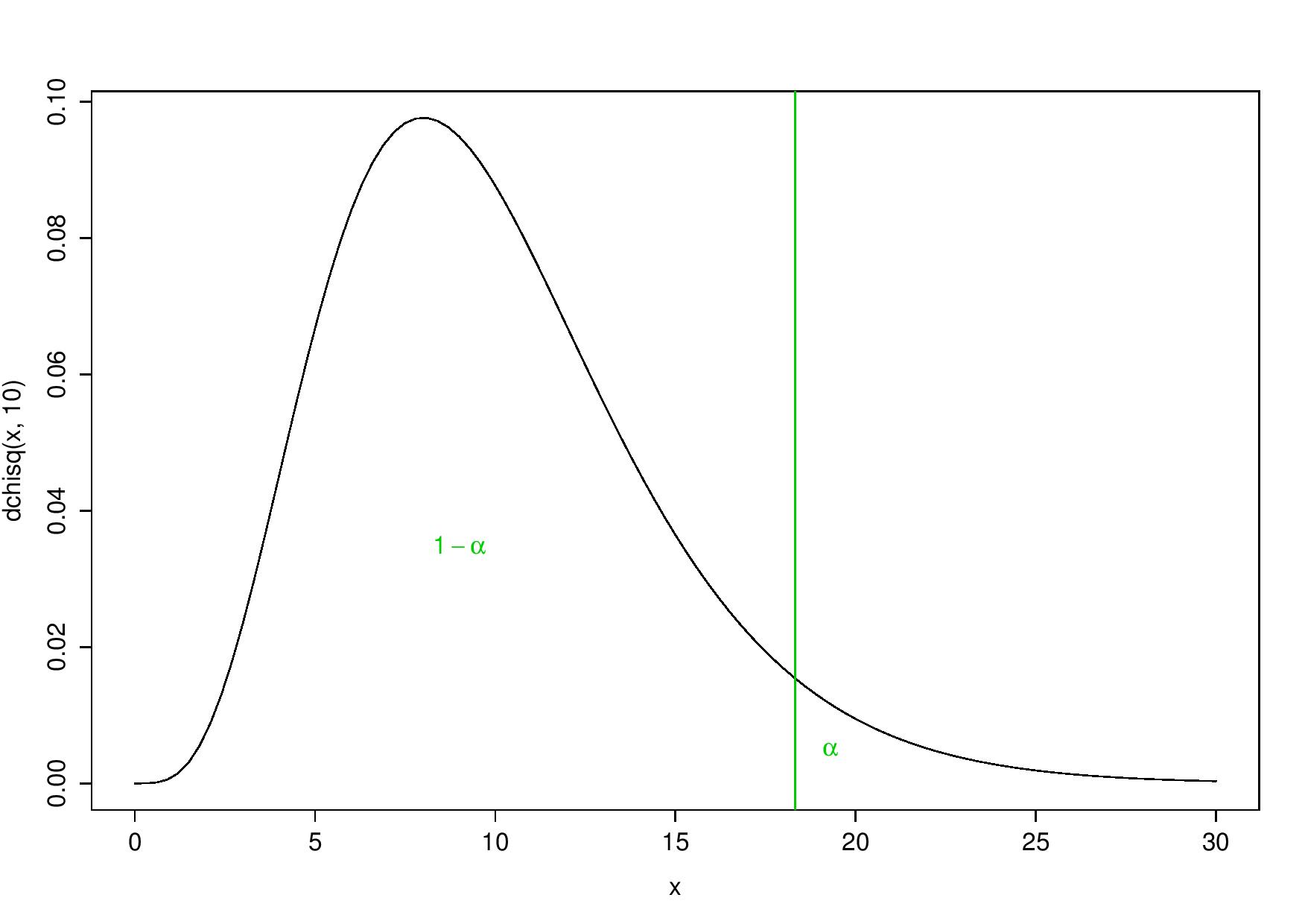
One-tailed test
- or to reject \(H_0\) for both largest and smallest values of the statistic. Indeed, smallest values could be considered “too good to be true” (Stuart 1954). Then, \(H_0\) is rejected for values smaller than the 2.5-percentile or larger than the 97.5-percentile:
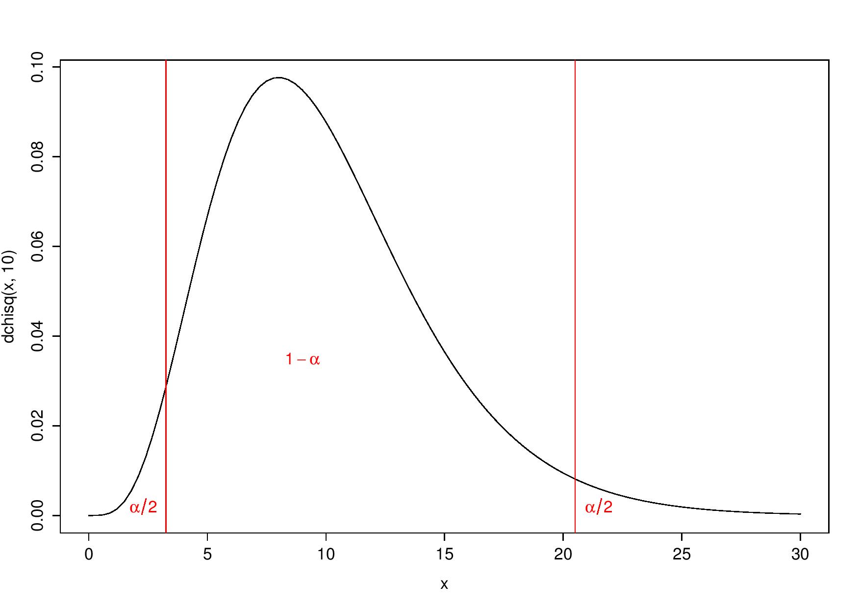
Two-tailed test
Why choosing? Why not letting the test choose by itself?
What do I mean by this? If you make the decision boundary on the test statistic’s density’s values (y-axis), not directly on the statistic’s values (x-axis), you always obtain a one-tailed test whatever is the distribution of the test statistic. Then, you reject \(H_0\) for all values that have a corresponding density lower than the 5-percentile:
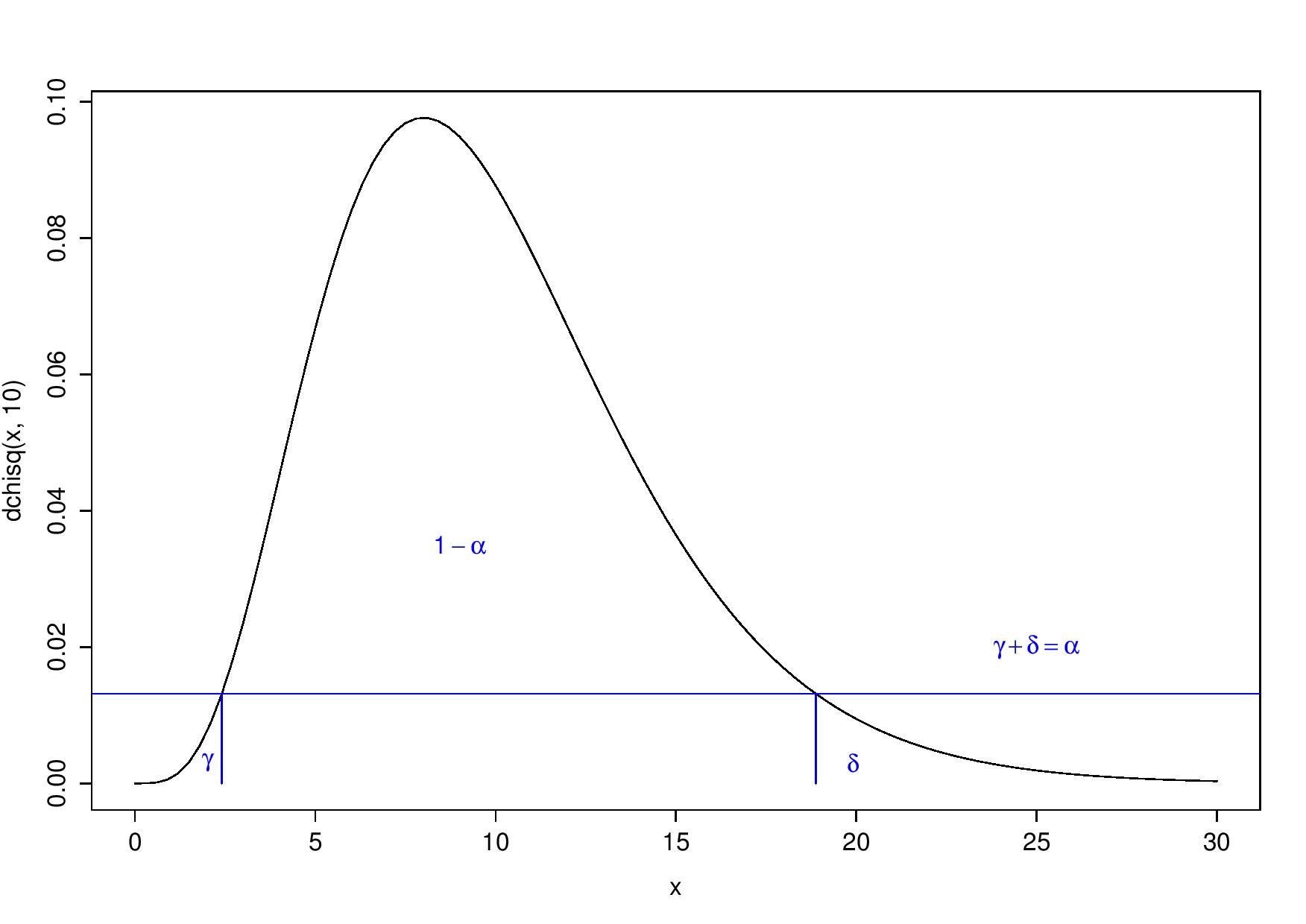
Always a one-tailed test, but with respect to the y-axis
I see this as rejecting the 5% less probable values (“probable” in terms of the test statistic’s density). This may be a way to get unbiased tests.
Application to the combination of tests
Combining tests may be a way to create more powerful or robust tests.
First example: application in reliability
Say that you have two goodness-of-fit test statistics for the Weibull distribution (GOFWs) (a well-known distribution in survival analysis). How to combine them?
A priori, the best way I can see is to use their joint distribution. A 2D distribution has a density, as before, so we can find a threshold so that only 5% of this distribution’s values have a corresponding density under this threshold. This threshold is also called a 95%-contour.
Again, an image will be clearer than words. I drew several samples of size 50 from the Weibull distribution and three alternatives to the Weibull distribution: the Gamma, Log-Normal and Dhillon I distributions. For all these samples, I computed the corresponding values of the two GOFWs, and I plotted these paired values:
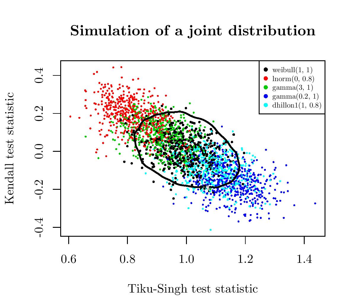
So, in black are the paired values for several samples of the Weibull distribution (the null hypothesis) and the alternatives are spread around. We have also in black the 95%-contour for \(H_0\). So, points outside of this boundary correspond to samples for which we reject the null hypothesis \(H_0\).
This gave one of the most powerful tests for the Weibull distribution.
For an example with R code, see the second example below.
Second example: application in genomics
Introduction
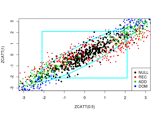
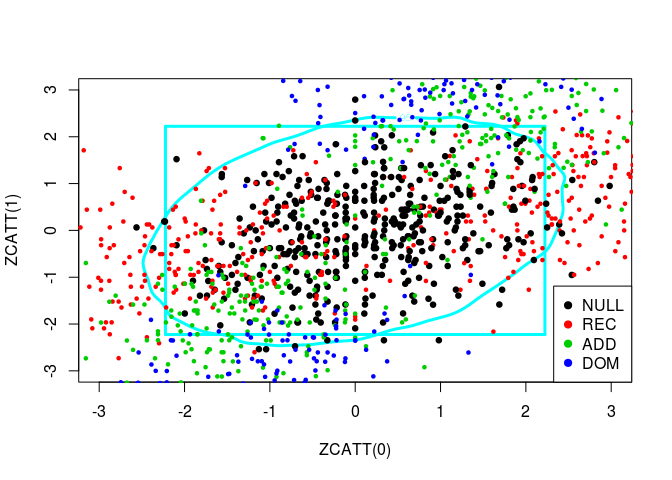
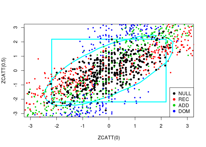
Cochran-Armitage Trend Tests (CATT) is well used in genomics to test for association between a single marker and a disease (Zheng et al. 2012, sec. 3.3.1). When the true genetic model is respectively the recessive (REC), additive (ADD), or dominant (DOM) model, the trend test ZCATT(x), where x is equal to 0, 1/2, or 1 respectively, gives powerful tests. Yet, the true model is generally unknown and choosing one specific value of x can lead to poor powers for some alternative models.
Then, the MAX3 statistic defined by \[MAX3 = \max\{|ZCATT(0)|, |ZCATT(1/2)|, |ZCATT(1)|\}\] can be used to have a more robust test (the power of the test remains good whatever is the underlying unkonwn model).
Yet, we could make another robust test based on the idea of the first section.
Simulation of values for these three statistics
I followed the algorithm detailed in (Zheng et al. 2012, sec. 3.9.1) to simulate contingency tables under different parameters as, for example, the genotype relative risk (GRR) \(\lambda_2\), the genetic model, the minor allele frequency (MAF) \(p\), etc.
source("../code/simu_counts.R")
source("../code/ZCATT.R")
Let us plot simulated values of three statistics, ZCATT(0), ZCATT(1/2) and ZCATT(1), by pairs. I will add to these plot two decision boundaries corresponding to the rejection of the null hypothesis for the statistics \(MAX2 = \max\{|S_1|, |S_2|\}\) (the square) and \(DENS2 = \hat{f}_{S_1, S_2}\) (the oval).
source("../code/square.R")
pacman::p_load(ks)

# Set of parameters
LWD <- 3; PCH <- 19; CEX <- 0.5
XLIM <- YLIM <-  c(-3, 3)
models <- c("NULL", "REC", "ADD", "DOM")
n <- length(models)
NSIM <- 200
lambda2 <- c(1.5, 1/1.5)
p <- 0.3

# Get lots of simulated values for the three statistics under H0
counts <- simu_counts(nsim = 1e5, p = p)
simus <- sapply(c(0, 0.5, 1), function(x) ZCATT(counts, x = x))
simus.save <- replace(simus, is.na(simus), 0)
colnames(simus.save) <- paste0("ZCATT(", c(0, 0.5, 1), ")")

# Plot by pairs
for (ind in -(1:3)) {
  simus2D <- simus.save[, ind]
  # DENS2
  k <- ks::kde(simus2D)
  plot(k, cont = 95, col = n+1, lwd = LWD,
       xlim = XLIM, ylim = YLIM)
  # MAX2
  q <- quantile(apply(abs(simus2D), 1, max), 0.95)
  square(q, col = 5, lwd = LWD)
  # H0 + Alternatives
  for (lam2 in lambda2) {
    for (i in 1:n) {
      counts <- simu_counts(nsim = NSIM, model = models[i],
                            lam2 = lam2, p = p)
      simus <- sapply(c(0, 0.5, 1), function(x) ZCATT(counts, x = x))
      simus <- replace(simus, is.na(simus), 0)[, ind]
      points(simus, col = i, cex = CEX, pch = PCH,
             lwd = ifelse(i == 1, LWD, 1))
    }
  }
  # Legend
  legend(x = "bottomright", legend = models, pch = PCH, col = 1:n)
}
Let us plot these three statistics’ values in 3D:
pacman::p_load(rgl, rglwidget)

rgl::plot3d(x = simus.save[1:NSIM, ], size = 5, xlab = "ZCATT(0)",
            ylab = "ZCATT(1/2)", zlab = "ZCATT(1)")
for (lam2 in lambda2) {
  for (i in 2:length(models)) {
    counts <- simu_counts(nsim = NSIM, p = p, model = models[i], lam2 = lam2)
    simus <- sapply(c(0, 0.5, 1), function(x) ZCATT(counts, x = x))
    rgl::plot3d(x = simus, col = i, add = TRUE)
  }
}
rglwidget()
We can see the three statistics’ values for the different models (H0: black, REC: red, ADD: green, DOM: blue) are almost on a same plane. So, it would be meaningless to estimate the 3D density.
Comparaison of MAX3 and this new idea
I rather projected these simulated values in 2D through a Principal Component Analysis and then made the new statistic with the 2D density of the first PCs:
  colnames(simus.save) <- NULL
  pca <- prcomp(simus.save, center = FALSE)
  simus2D <- pca$x[, 1:2]
  # DENS2 on PCs
  k <- ks::kde(simus2D)
  plot(k, cont = 95, col = n+1, lwd = LWD)
  # MAX3
  q <- quantile(apply(abs(simus.save), 1, max), 0.95)
  for (j in 1:3) {
    cart <- pca$rotation[j, 1:2]
    abline(q/cart[2], -cart[1]/cart[2], col = j+1)
    abline(-q/cart[2], -cart[1]/cart[2], col = j+1)
  }
  legend(x = "topright", legend = paste0("ZCATT(", c(0, 0.5, 1), ")"),
         lwd = 1, col = 2:4)
  # H0 + Alternatives
  for (lam2 in lambda2) {
    for (i in 1:n) {
      counts <- simu_counts(nsim = NSIM, model = models[i],
                            lam2 = lam2, p = p)
      simus <- sapply(c(0, 0.5, 1), function(x) ZCATT(counts, x = x))
      simus <- replace(simus, is.na(simus), 0)
      simus <- predict(pca, simus)
      points(simus, col = i, cex = CEX, pch = PCH,
             lwd = ifelse(i == 1, LWD, 1))
    }
  }
  # Legend
  legend(x = "bottomright", legend = models, pch = PCH, col = 1:n)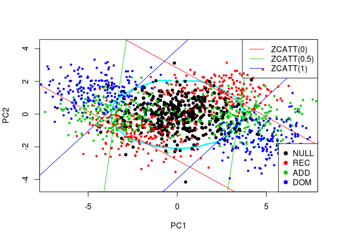
The lines correspond to the decision boundaries of MAX3: for each of the 3 studied statistic, \(H_0\) is rejected for a point which is outside the corresponding two lines. At this point, if I made myself clear enough, you should see that the decision boundary of MAX3 on the previous plot is defined by the convex hull of the 6 lines.
As before, the oval represents the DENS2 statistic (here, on the two first PCs). It does give a robust test, yet slightly less powerful than MAX3. Indeed, to compare these two tests, there is no need for computing their precise powers for each alternative. You just have to compare the number of alternatives (blue, green, and red points) for which \(H_0\) is rejected with one test but not the other, on the plot. At the top and bottom of the plot, we can see a large region where we would reject \(H_0\) with DENS2 and not MAX3, yet there are not many alternatives in there. On the contrary, there are 3 small areas on the left and on the right of the plot where we would reject \(H_0\) with MAX3 and not DENS2, yet there are many alternatives in there.
The problem of DENS2 being slightly less powerful, I think, is that the 2D or 3D distributions of the statistics’ values for the alternatives are highly correlated with the ones of the null hypothesis (they have the same shape and tends to be on the same diagonal). So, even if the “area of H0” is larger with MAX2 or MAX3 than DENS2 (see all 2D plots), the number of alternatives in there is lower, so they give a more powerful test than DENS2 in this case.
Conlusion
We have seen how to use density to get robust and powerful tests, without any subjective choice. We have also visualized some combination of tests and directly assessed from plots the powers of tests for multiple alternatives. Yet, we have not seen how DENS1 could unbias tests (you should try it yourself).
In practice, this works well with approximately normally distributed statistics because it’s then easy to get a non-parametric estimation of the density via the use of a Gaussian Kernel (what does kde).
References
Stuart, Alan. 1954. “Too Good to Be True?” Journal of the Royal Statistical Society. Series C (Applied Statistics) 3 (1). [Wiley, Royal Statistical Society]: 29–32. http://www.jstor.org/stable/2985442.
Zheng, Gang, Yaning Yang, Xiaofeng Zhu, and Robert C. Elston. 2012. Analysis of Genetic Association Studies. Statistics for Biology and Health. Boston, MA: Springer US. doi:10.1007/978-1-4614-2245-7.