Detecting outlier samples in PCA
In this post, I present something I am currently investigating (feedback welcome!) and that I am implementing in my new package {bigutilsr}. This package can be used to detect outlier samples in Principal Component Analysis (PCA).
remotes::install_github("privefl/bigutilsr")library(bigutilsr)I present three different statistics of outlierness and two different ways to choose the threshold of being an outlier for those statistics.
A standard way to detect outliers
Data
X <- readRDS(system.file("testdata", "three-pops.rds", package = "bigutilsr"))
pca <- prcomp(X, scale. = TRUE, rank. = 10)
U <- pca$xlibrary(ggplot2)
theme_set(bigstatsr::theme_bigstatsr(0.8))
qplot(U[, 1], U[, 2]) + coord_equal()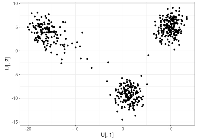
Measuring outlierness
The standard way to detect outliers in genetics is the criterion of being “more than 6 standard deviations away from the mean”.
apply(U, 2, function(x) which( abs(x - mean(x)) > (6 * sd(x)) ))## integer(0)Here, there is no outlier according to this criterion. Let us make some fake one.
U2 <- U
U2[1, 1] <- 30
qplot(U2[, 1], U2[, 2]) + coord_equal()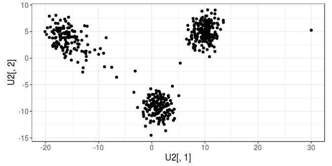
apply(U2, 2, function(x) which( abs(x - mean(x)) > (6 * sd(x)) ))## integer(0)Still not an outlier..
U3 <- U2
U3[1, 1] <- 80
qplot(U3[, 1], U3[, 2]) + coord_equal()
library(magrittr)
apply(U3, 2, function(x) which( abs(x - mean(x)) > (6 * sd(x)) )) %>%
  Reduce(union, .)
## [1] 1Now, the first sample is considered as an outlier by this criterion.
A more robust variation
Note that you might want to use median() instead of mean() and mad() instead of sd() because they are more robust estimators. This becomes
ind.out <- apply(U3, 2, function(x) which( (abs(x - median(x)) / mad(x)) > 6 )) %>%
  Reduce(union, .) %>%
  print()
## [1] 1 516We get a new outlier.
col <- rep("black", nrow(U3)); col[ind.out] <- "red"
qplot(U3[, 1], U3[, 3], color = I(col), size = I(2)) + coord_equal()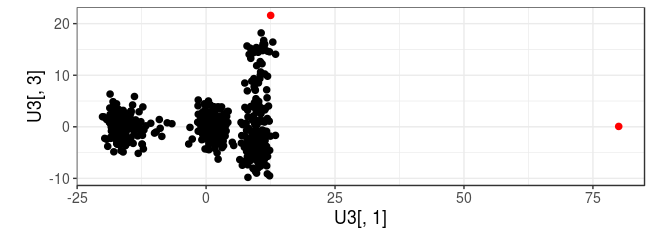
A continuous view of this criterion
This criterion flag an outlier if it is an outlier for at least one principal component (PC). This corresponds to using the max() (infinite) distance (in terms of number of standard deviations) from the mean.
dist <- apply(U3, 2, function(x) abs(x - median(x)) / mad(x)) %>%
  apply(1, max)
qplot(U3[, 1], U3[, 3], color = dist, size = I(3)) + coord_equal() +
  scale_color_viridis_c(trans = "log", breaks = c(1, 3, 6))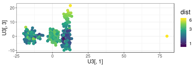
qplot(y = sort(dist, decreasing = TRUE)) +
  geom_hline(yintercept = 6, color = "red")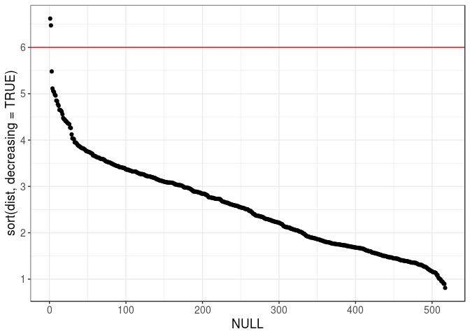
Investigating two other criteria of outlierness
Robust Mahalanobis distance
Instead of using the infinite distance, Mahalanobis distance is a multivariate distance based on all variables (PCs here) at once. We use a robust version of this distance, which is implemented in packages {robust} and {robustbase} (Gnanadesikan and Kettenring 1972, Yohai and Zamar (1988), Maronna and Zamar (2002), Todorov, Filzmoser, and others (2009)) and that is reexported in {bigutilsr}.
dist2 <- covRob(U3, estim = "pairwiseGK")$dist
qplot(dist, sqrt(dist2))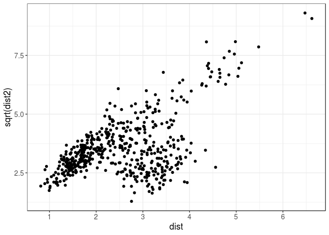
cowplot::plot_grid(
  qplot(U3[, 1], U3[, 2], color = dist2, size = I(2)) + coord_equal() +
    scale_color_viridis_c(trans = "log", breaks = NULL),
  qplot(U3[, 3], U3[, 7], color = dist2, size = I(2)) + coord_equal() +
    scale_color_viridis_c(trans = "log", breaks = NULL),
  rel_widths = c(0.7, 0.4), scale = 0.95
)
This new criterion provides similar results for this data. These robust Mahalanobis distances are approximately Chi-square distributed, which enables deriving p-values of outlierness.
pval <- pchisq(dist2, df = 10, lower.tail = FALSE)
hist(pval)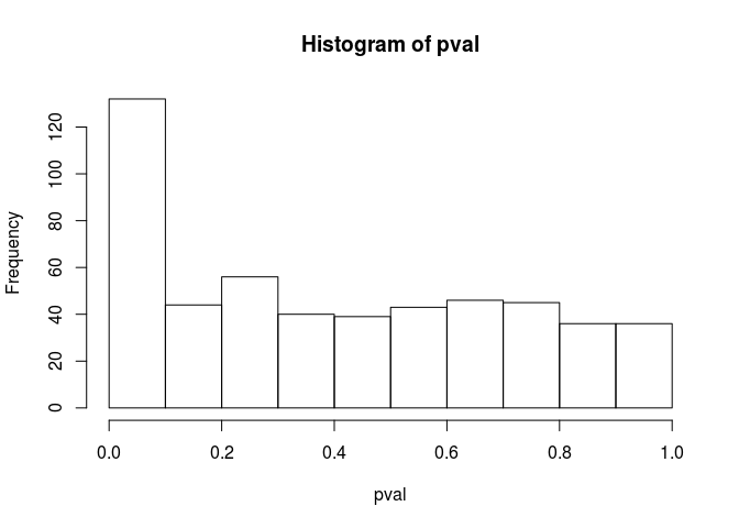
is.out <- (pval < (0.05 / length(dist2)))  # Bonferroni correction
sum(is.out)
## [1] 33qplot(U3[, 3], U3[, 7], color = is.out, size = I(3)) + coord_equal()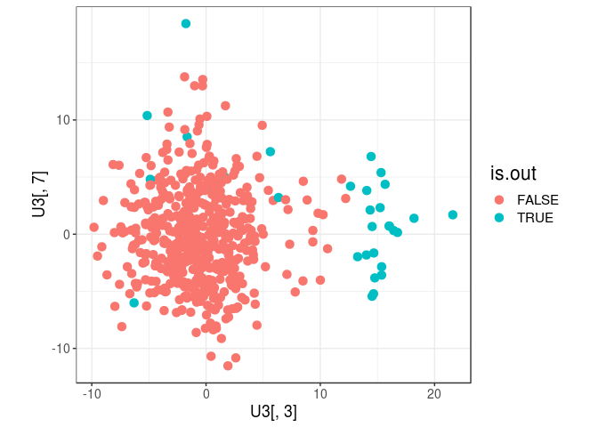
Local Outlier Factor (LOF)
LOF statistic (Breunig et al. 2000) has been cited more than 4000 times. Instead of computing a distance from the center, it uses some local density of points. We make use of the fast K nearest neighbours implementation of R package {nabor} (Elseberg et al. 2012) to implement this statistic efficiently in {bigutilsr}.
llof <- LOF(U3)  # log(LOF) by default
qplot(dist2, llof)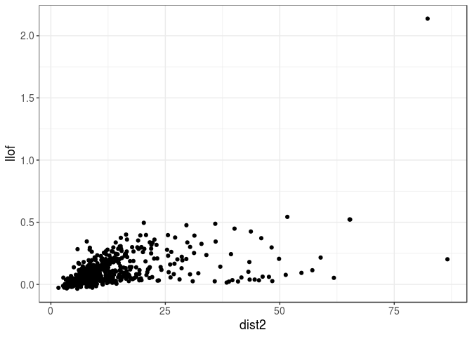
The fake outlier that we introduced is now clearly an outlier. The other points, not so much.
cowplot::plot_grid(
  qplot(U3[, 1], U3[, 2], color = llof, size = I(3)) + coord_equal() +
    scale_color_viridis_c(breaks = NULL),
  qplot(U3[, 3], U3[, 7], color = llof, size = I(3)) + coord_equal() +
    scale_color_viridis_c(breaks = NULL),
  rel_widths = c(0.7, 0.4), scale = 0.95
)
Choosing the threshold of being an outlier
Threshold of 6 for the first criterion presented here may appear arbitrary. If the data you have is normally distributed, each sample (for each PC) has a probability of 2 * pnorm(-6) (2e-9) of being considered as an outlier by this criterion.
Accounting for multiple testing, for 10K samples and 10 PCs, there is a chance of 1 - (1 - 2 * pnorm(-6))^100e3 (2e-4) of detecting at least one outlier. If choosing 5 as threshold, there is 5.6% chance of detecting at least one outlier when PCs are normally distributed. If choosing 3 instead, this probability is 1.
Tukey’s rule
Tukey’s rule (Tukey 1977) is a standard rule for detecting outliers. Here, we will apply it on the previously computed statistics. Note that we could use it directly on PCs, which is not much different from the robust version of the first criterion we introduced.
x <- rnorm(10000)
(tukey_up  <- quantile(x, 0.75) + 1.5 * IQR(x))
## 75%
## 2.70692(tukey_low <- quantile(x, 0.25) - 1.5 * IQR(x))## 25%
## -2.725665hist(x); abline(v = c(tukey_low, tukey_up), col = "red")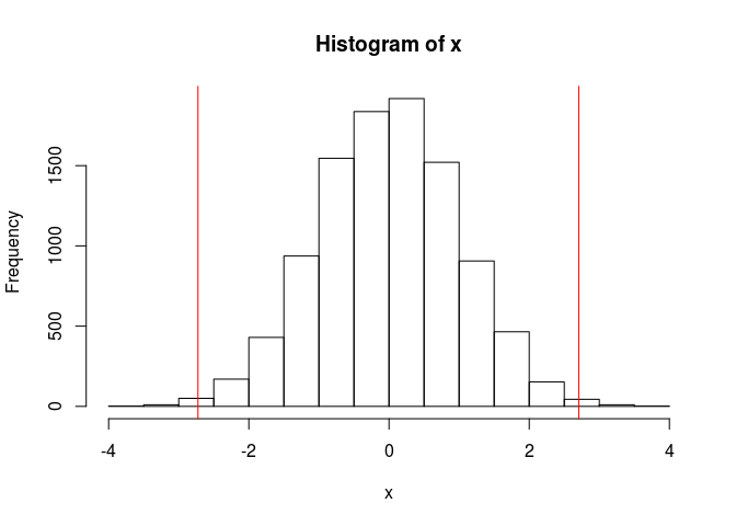
mean(x < tukey_low | x > tukey_up)## [1] 0.0057where IQR(x) is equal to quantile(x, 0.75) - quantile(x, 0.25) (the InterQuartile Range).
However, there are two pitfalls when using Tukey’s rule:
Tukey’s rule assumes a normally distributed sample. When the data is skewed, it does not work that well.
x <- rchisq(10000, df = 5)
(tukey_up  <- quantile(x, 0.75) + 1.5 * IQR(x))
## 75% ## 12.42084(tukey_low <- quantile(x, 0.25) - 1.5 * IQR(x))## 25% ## -3.232256hist(x, "FD"); abline(v = c(tukey_low, tukey_up), col = "red")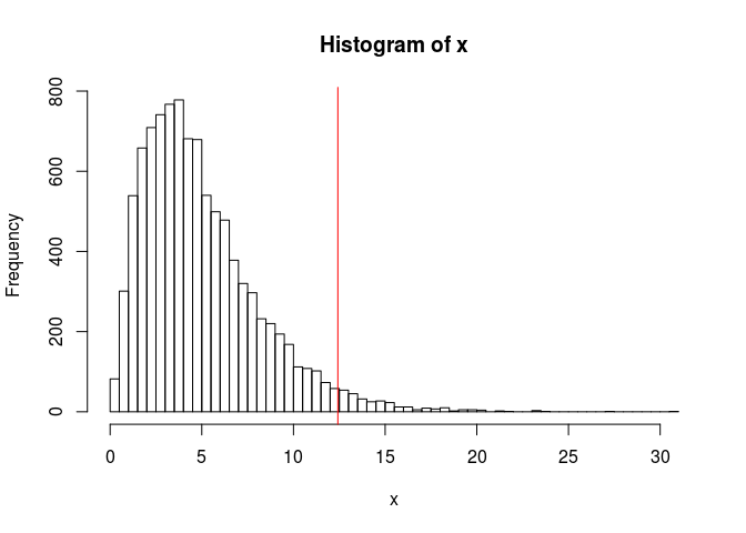
mean(x < tukey_low | x > tukey_up)## [1] 0.0294To solve the problem of skewness, the medcouple (mc) has been introduced (Hubert and Vandervieren 2008) and is implemented in
robustbase::adjboxStats().Tukey’s rule uses a fixed coefficient (
1.5) that does not account for multiple testing, which means that for large samples, you will almost always get some outliers if using1.5.
To solve these two issues, we implemented tukey_mc_up() that accounts both for skewness and multiple testing by default.
x <- rchisq(10000, df = 5)
(tukey_up  <- quantile(x, 0.75) + 1.5 * IQR(x))
## 75%
## 12.48751hist(x, "FD"); abline(v = tukey_up, col = "red")
abline(v = print(tukey_mc_up(x, coef = 1.5)), col = "blue")## [1] 16.74215abline(v = print(tukey_mc_up(x)), col = "green") # accounts for multiple testing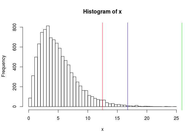
## [1] 25.93299Applying this corrected Tukey’s rule to our statistics:
tukey_mc_up(dist)## [1] 6.406337qplot(dist2, llof) +
geom_vline(xintercept = tukey_mc_up(dist2), color = "red") +
geom_hline(yintercept = tukey_mc_up(llof), color = "red")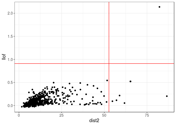
Histogram’s gap
This rule I come up with assumes that the “normal” data is somewhat grouped and the outliers have some gap (in the histogram, there is a bin with no value in it) with the rest of the data.
For example, for dist, there is a gap just before 6, and we can derive an algorithm to detect this:
hist(dist, breaks = nclass.scottRob)
str(hist_out(dist))
## List of 2
## $ x : num [1:515] 2.08 2.06 1.74 1.86 2.04 ...
## $ lim: num [1:2] -Inf 5.75abline(v = hist_out(dist)$lim[2], col = "red")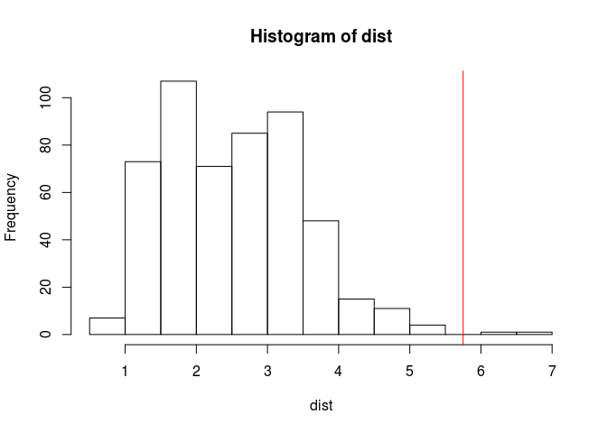
hist(dist2, breaks = nclass.scottRob)
abline(v = hist_out(dist2)$lim[2], col = "red")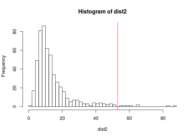
hist(llof, breaks = nclass.scottRob)
abline(v = hist_out(llof)$lim[2], col = "red")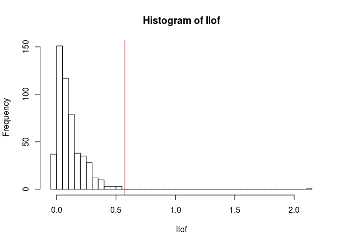
This criterion is convenient because it does not assume any distribution of the data, just that it is compact and that the outliers are not in the pack.
It could be used in other contexts, e.g. choosing the number of outlier principal components:
eigval <- pca$sdev^2
hist(eigval, breaks = "FD")  # "FD" gives a bit more bins than scottRob
abline(v = hist_out(eigval, breaks = "FD")$lim[2], col = "red")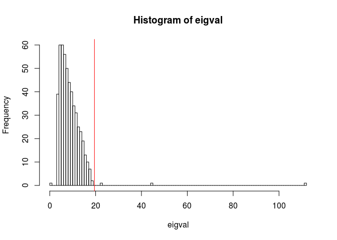
sum(eigval > hist_out(eigval, breaks = "FD")$lim[2])## [1] 3pca_nspike(eigval) # directly implemented in {bigutilsr}## [1] 3Note the possible use of bootstrap to make hist_out() and pca_nspike() more robust.
Conclusion
Outlier detection is not an easy task, especially if you want the criterion of outlierness to be robust to several factors such as sample size and distribution of the data. Moreover, there is always some threshold to choose to separate outliers from non-ouliers.
With one small example, we have seen several statistics to compute some degree of outlierness:
- “6 standard deviations away from the mean” that somewhat assumes that PCs are normally distributed. Here, data is more a mixture of distributions (one for each cluster) than one normal distribution so that it might not work that well.
- Mahalanobis distance that also assumes a (multivariate) normal distribution but that takes into account the correlation between PCs (that is not the identity because we use a robust estimation).
- Local Outlier Factor (LOF) that does not assume any distribution and that finds points that are in empty areas (far from every other points) rather than points that are far from the center. One drawback is that this statistic has an hyper-parameter K (nearest neighbours); we combine three different values by default to make this statistic more robust to the choice of this parameter K.
and several ways to decide the threshold of being an outlier according to those statistics:
- Tukey’s rule, adjusting for skewness and multiple testing.
- “Histogram’s gap” that finds a gap between outlier values and “normal” values based on a histogram.
I have been investigating outlier detection in the past weeks. Any feedback and further input on this would be great.
References
Breunig, Markus M, Hans-Peter Kriegel, Raymond T Ng, and Jörg Sander. 2000. “LOF: Identifying Density-Based Local Outliers.” In ACM Sigmod Record, 29:93–104. 2. ACM.
Elseberg, Jan, Stéphane Magnenat, Roland Siegwart, and Andreas Nüchter. 2012. “Comparison of Nearest-Neighbor-Search Strategies and Implementations for Efficient Shape Registration.” Journal of Software Engineering for Robotics 3 (1): 2–12.
Gnanadesikan, Ramanathan, and John R Kettenring. 1972. “Robust Estimates, Residuals, and Outlier Detection with Multiresponse Data.” Biometrics. JSTOR, 81–124.
Hubert, Mia, and Ellen Vandervieren. 2008. “An Adjusted Boxplot for Skewed Distributions.” Computational Statistics & Data Analysis 52 (12). Elsevier: 5186–5201.
Maronna, Ricardo A, and Ruben H Zamar. 2002. “Robust Estimates of Location and Dispersion for High-Dimensional Datasets.” Technometrics 44 (4). Taylor & Francis: 307–17.
Todorov, Valentin, Peter Filzmoser, and others. 2009. “An Object-Oriented Framework for Robust Multivariate Analysis.” Citeseer.
Tukey, John W. 1977. Exploratory Data Analysis. Addison-Wesley.
Yohai, Victor J, and Ruben H Zamar. 1988. “High Breakdown-Point Estimates of Regression by Means of the Minimization of an Efficient Scale.” Journal of the American Statistical Association 83 (402). Taylor & Francis: 406–13.