Using clustering to find points in an image

Written on November 27, 2018

In this post, I present my new package {img2coord}. This package can be used to retrieve coordinates from a scatter plot (as an image).

devtools::install_github("privefl/img2coord")

Have you ever made a plot, saved it as a png and moved on? When you come back to it, it is sometimes difficult to read the values from this plot, especially if there is no grid inside the plot.
Making this package was also a good way to practice with clustering.

A very simple example

Saving a plot as PNG

file <- tempfile(fileext = ".png")
png(file, width = 600, height = 400)
set.seed(1)
plot(c(0, runif(20), 1))
dev.off()

## png 
##   2

Reading the PNG in R

(img <- magick::image_read(file))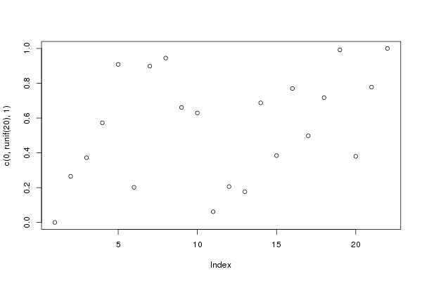

Get pixel indices from points

## grayscale
img_mat <- img2coord:::img2mat(img)
dim(img_mat)

## [1] 400 600

list.contour <- img2coord:::get_contours(img_mat)
img_mat_in <- img2coord:::get_inside(img_mat, list.contour)
dim(img_mat_in)

## [1] 264 507

head(ind <- which(img_mat_in > 0, arr.ind = TRUE))

##      row col
## [1,] 256  14
## [2,] 257  14
## [3,] 254  15
## [4,] 255  15
## [5,] 256  15
## [6,] 257  15

Cluster pixel indices

set.seed(1)
km <- kmeans(ind, centers = 22)

library(ggplot2)
myplot <- function(points, centers) {
  p <- ggplot() + 
    geom_tile(aes(col, row), data = as.data.frame(points)) + 
    geom_point(aes(col, row), data = as.data.frame(centers), col = "red") + 
    bigstatsr::theme_bigstatsr() + 
    coord_equal()
  print(p)
}
myplot(ind, km$centers)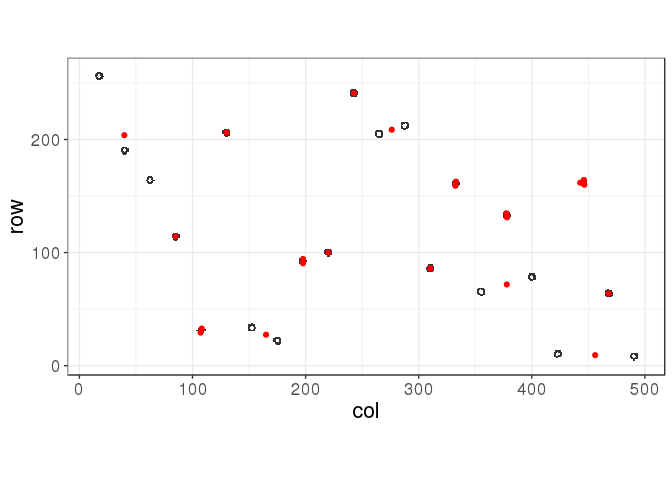

Even when using the true number of clusters, kmeans get trapped in a local minimum (this is clearly not the best solution!), depending on the initialisation of centers. One possible solution would be to use many initialisations; let’s try that.

set.seed(1)
km <- kmeans(ind, centers = 22, nstart = 100, iter.max = 100)

## Warning: did not converge in 100 iterations

## Warning: did not converge in 100 iterations

myplot(ind, km$centers)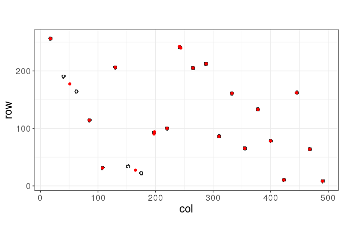

It is better but not optimal.

Using hclust to get centers

get_centers <- function(points, clusters) {
  do.call("rbind", by(points, clusters, colMeans, simplify = FALSE))
}

d <- dist(ind)
hc <- hclust(d)
centers <- get_centers(ind, cutree(hc, k = 22))
myplot(ind, centers)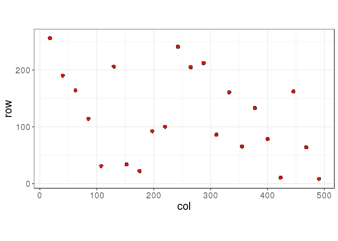

hclust() works well for this example.

Get the number of clusters

What if we don’t know the number of clusters (representing the initial points)? A statistic that could help us determine the number of clusters to use is the silhouette.

K_seq <- seq(10, 30)
stat <- sapply(K_seq, function(k) {
  mean(cluster::silhouette(cutree(hc, k), d)[, 3])
})
plot(K_seq, stat, pch = 20); abline(v = 22, lty = 3)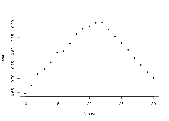

A less simple example

file <- tempfile(fileext = ".png")
png(file, width = 600, height = 400)
set.seed(1)
y <- c(0, runif(100), 1)
plot(y, cex = runif(102, min = 0.5, max = 1.5))
dev.off()

## png 
##   2

(img <- magick::image_read(file))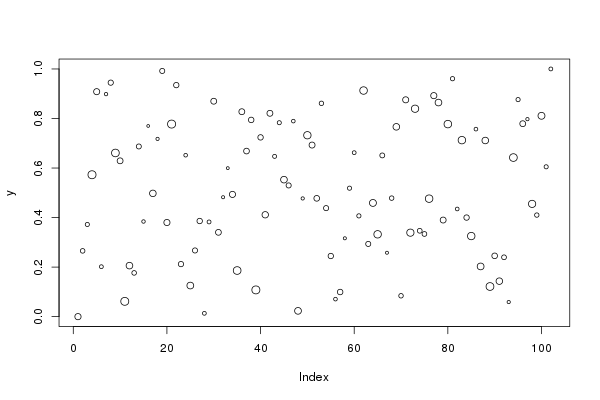

img_mat <- img2coord:::img2mat(img)
list.contour <- img2coord:::get_contours(img_mat)
img_mat_in <- img2coord:::get_inside(img_mat, list.contour)
ind <- which(img_mat_in > 0, arr.ind = TRUE)

hc <- flashClust::hclust(d <- dist(ind))
K_seq <- seq(50, 150)
stat <- sapply(K_seq, function(k) {
  mean(cluster::silhouette(cutree(hc, k), d)[, 3])
})
plot(K_seq, stat, pch = 20); abline(v = 102, lty = 3)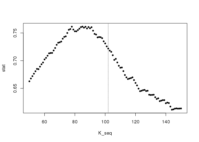

(K_opt <- K_seq[which.max(stat)])

## [1] 85

centers <- get_centers(ind, cutree(hc, k = K_opt))
myplot(ind, centers)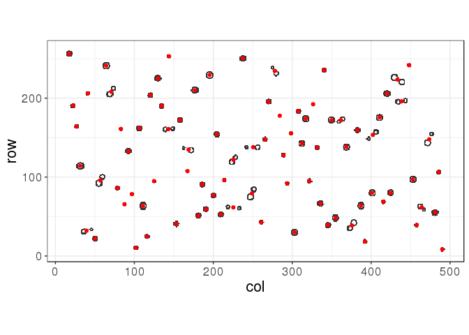

The silhouette statistic is giving a good yet not optimal solution in this situation. Using the true number of points, we would get:

centers <- get_centers(ind, cutree(hc, k = 102))
myplot(ind, centers)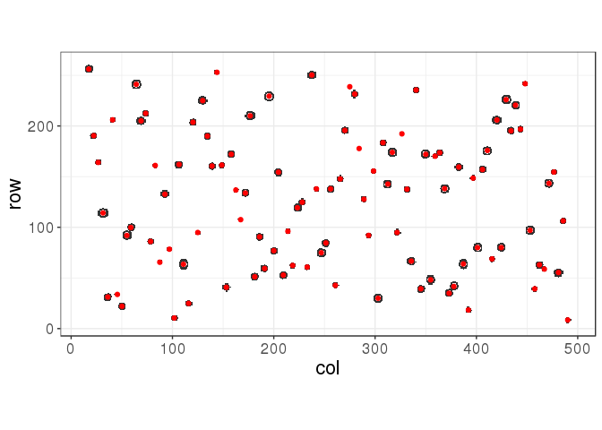

If someone has a better statistic to (automatically) find the number of clusters, please share it and I’ll update this post.

Putting everything together as a package

Finally, after you get the center of all points (pixel clusters), you can interpolate the values based on the values of axe ticks.

coord <- img2coord::get_coord(
  file, 
  x_ticks = seq(0, 100, 20),
  y_ticks = seq(0, 1, 0.2),
  K_min = 50, K_max = 150
)

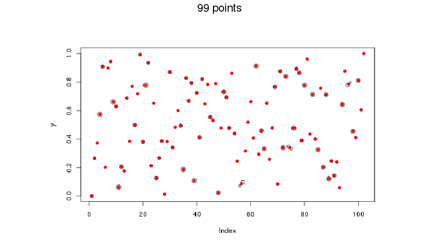
This works better here because I combined the silhouette statistic with a gini coefficient (measure of dispersion) of the number of pixels in each cluster (assuming that they should have approximately the same number). Let’s have a look at the combined statistic:

stat <- attr(coord, "stat")
plot(names(stat), stat, pch = 20); abline(v = 102, lty = 3)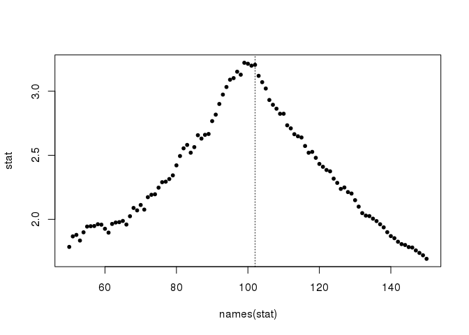

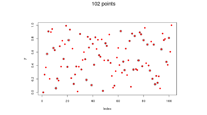
If you don’t get the right number of clusters the first time, you can use the plot generated by img2coord::get_coord() to adjust K.

coord <- img2coord::get_coord(
  file, 
  x_ticks = seq(0, 100, 20),
  y_ticks = seq(0, 1, 0.2),
  K = 102  ## 99 + 3
)

Let’s verify the coordinates we get:

round(coord$x, 2)

##   [1]   1.00   2.01   3.01   4.00   4.99   6.01   7.00   8.00   9.01  10.01
##  [11]  10.98  11.99  12.99  14.01  15.00  15.98  17.01  18.00  18.98  20.00
##  [21]  20.99  22.00  23.00  23.99  24.98  26.00  26.99  28.01  29.00  29.98
##  [31]  31.01  31.99  33.02  34.00  35.02  35.98  37.00  38.01  38.99  40.00
##  [41]  40.99  41.99  42.99  44.01  44.97  45.98  47.01  48.00  49.00  50.00
##  [51]  51.01  51.98  52.99  53.99  55.00  56.00  57.01  58.01  59.00  60.02
##  [61]  61.00  62.00  62.98  64.01  64.99  65.98  67.00  68.01  68.98  70.00
##  [71]  70.98  72.00  73.00  74.01  75.00  76.01  77.00  78.00  79.02  79.98
##  [81]  81.00  82.01  82.98  84.00  85.01  85.99  87.01  87.98  88.99  89.99
##  [91]  90.98  92.00  93.00  94.01  95.00  95.89  96.87  97.99  99.00 100.00
## [101] 101.01 101.99

plot(coord$y, y, pch = 20); abline(0, 1, col = "red")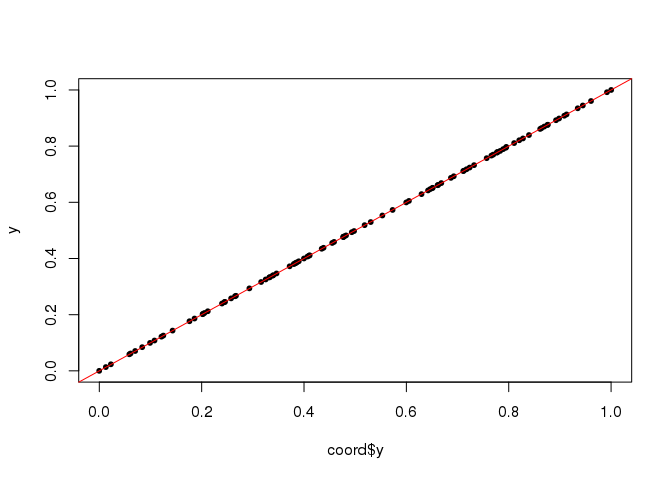

Handling large images

url <- "https://goo.gl/K6Y7D1"
library(img2coord)
(img <- img_read(url))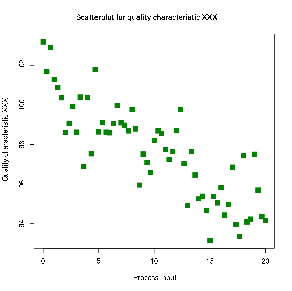

get_coord(img, seq(0, 20, 5), seq(94, 102, 2), K_min = 40, K_max = 80)

## Error: Detected more than 10000 pixels associated with points (21358).
##   Make sure you have a white background with no grid (only points).
##   You can change 'max_pixels', but it could become time/memory consuming.
##   You can also downsize the image using `img_scale()`.

The green points are spanning 21,358 pixels, which could be a lot to process, depending on your computer. To solve this problem, you can do:

img %>%
 img_scale(0.4) %>%
 get_coord(seq(0, 20, 5), seq(94, 102, 2), K_min = 40, K_max = 80)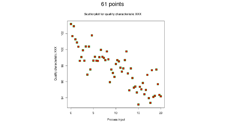

## $x
##  [1] -0.0005401687  0.3343468897  0.6664667098  0.9992303467  1.3337481120
##  [6]  1.6671560578  1.9997172265  2.3332269701  2.6674887594  2.9991939098
## [11]  3.3326859175  3.6672015650  4.0000566377  4.3329094030  4.6674459579
## [16]  5.0009192485  5.3326185095  5.6478368286  6.0464367945  6.3329501844
## [21]  6.6663573828  6.9839799351  7.3513525635  7.6674682785  8.0006621331
## [26]  8.3329974666  8.6657575234  8.9999189758  9.3339407034  9.6666009658
## [31] 10.0001231324 10.3173252500 10.6778169496 10.9989528978 11.3335964907
## [36] 11.6665738876 11.9994145980 12.3336165187 12.6676553366 12.9992455320
## [41] 13.3331964821 13.6668686496 13.9813979399 14.3425396058 14.6672323938
## [46] 15.0002253318 15.3330976683 15.6669750015 16.0007098735 16.3322818494
## [51] 16.6663301257 17.0005035442 17.3333809139 17.6663416006 18.0009680691
## [56] 18.3172429708 18.6798897677 18.9998067488 19.3333374006 19.6570288544
## [61] 20.0116006657
## 
## $y
##  [1] 103.18007 101.68089 102.91175 101.28109 100.89144 100.36108  98.59931
##  [8]  99.06933  99.90900  98.61988 100.39017  96.87960 100.38054  97.52969
## [15] 101.77948  98.63014  99.10885  98.62457  98.58221  99.06001  99.97088
## [22]  99.09976  98.96014  98.68939  99.77109  98.78963  95.94976  97.51865
## [29]  97.07733  96.58967  98.21105  98.69922  98.53481  97.74167  97.24962
## [36]  97.65023  98.70168  99.77109  97.02095  94.91963  97.65023  96.46068
## [43]  95.23798  95.39595  94.64729  93.14815  95.35968  95.04774  95.82991
## [50]  94.43923  94.96829  96.84944  93.94962  93.35852  97.42928  94.07914
## [57]  94.23708  97.51029  95.68894  94.35497  94.16229
## 
## attr(,"stat")
##        40        41        42        43        44        45        46 
##  1.991872  2.074327  2.140775  2.270267  2.341965  2.529008  2.758398 
##        47        48        49        50        51        52        53 
##  2.920247  3.119059  3.244979  3.377485  3.715905  4.083564  4.563417 
##        54        55        56        57        58        59        60 
##  5.104999  5.841044  6.441349  6.551265  7.246189  8.165916  8.842711 
##        61        62        63        64        65        66        67 
## 10.167292  8.357433  6.887889  5.708635  4.889674  4.274374  3.788661 
##        68        69        70        71        72        73        74 
##  3.384619  3.082882  2.836479  2.630589  2.451460  2.292444  2.162840 
##        75        76        77        78        79        80 
##  2.054934  1.947805  1.870104  1.784646  1.701550  1.630990

Conclusion

We have seen that hclust() was performing better than kmeans() (for this example). For some reason I don’t understand yet, initializing kmeans() with centers from hclust() works even better.

Then, we have seen how to determine the number of clusters. Finally, we have seen that using a particular statistic, specifically designed for this problem, improved the solution.

Of course, this could be improved a lot. For example, this won’t work for plots having a background color or some grid inside. Feel free to bring your ideas. BTW, thanks Robin who brought some nice ideas that improved this package a lot.

Have a look at the GitHub repo.