Plot method

Plot method for class big_SVD.

# S3 method for big_SVD
plot(
  x,
  type = c("screeplot", "scores", "loadings"),
  nval = length(x$d),
  scores = c(1, 2),
  loadings = 1,
  ncol = NULL,
  coeff = 1,
  viridis = TRUE,
  cols = 2,
  ...
)

Arguments

x

An object of class big_SVD.

type

Either

"screeplot": plot of decreasing singular values (the default).
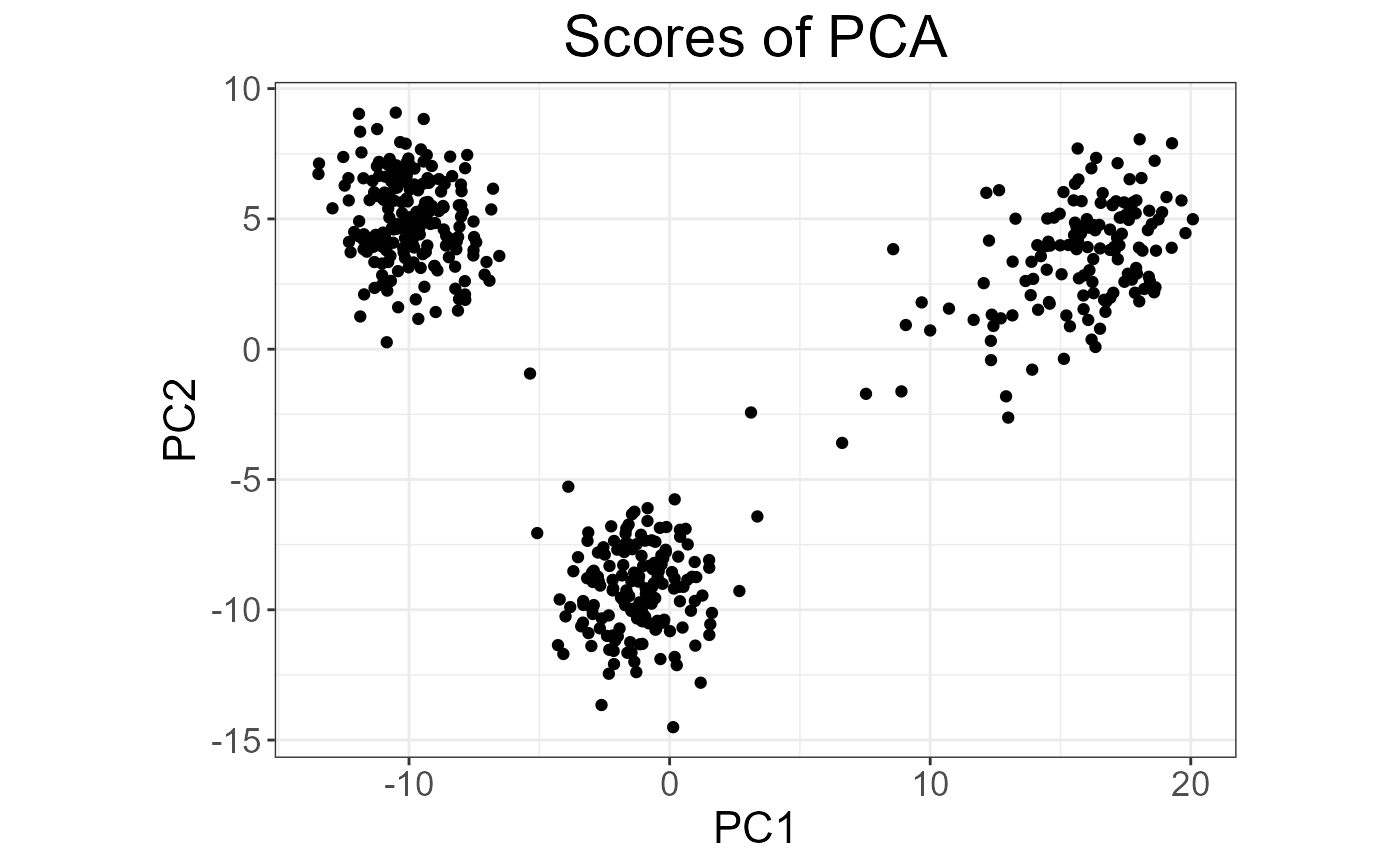
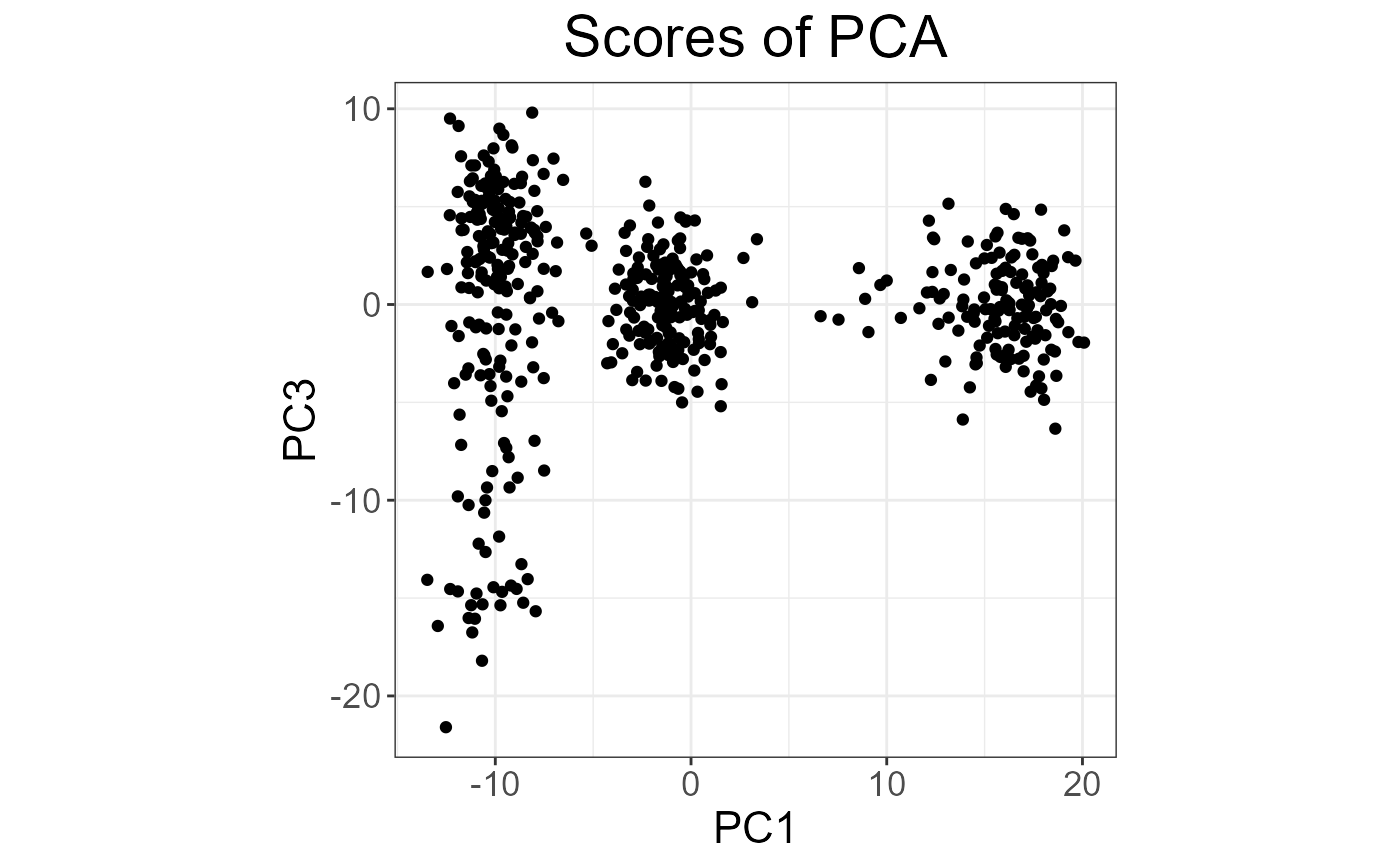
"scores": plot of the scores associated with 2 Principal Components.
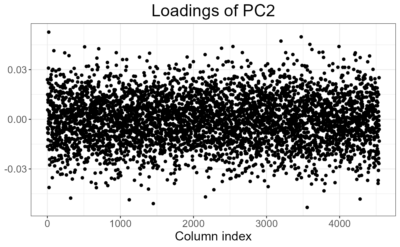
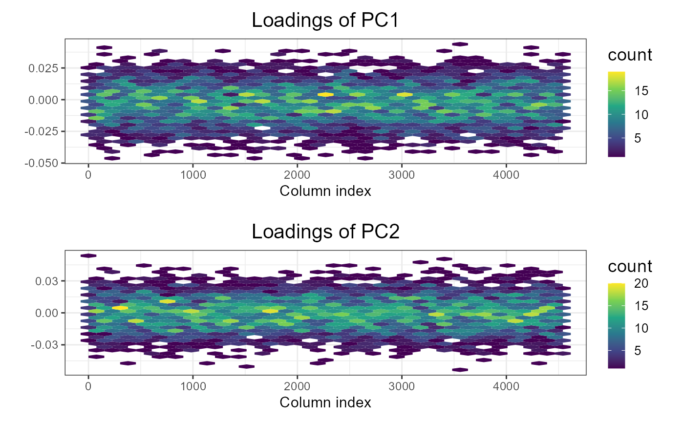
"loadings": plot of loadings associated with 1 Principal Component.

nval

Number of singular values to plot. Default plots all computed.

scores

Vector of indices of the two PCs to plot. Default plots the first two PCs. If providing more than two, it produces many plots.

loadings

Indices of PC loadings to plot. Default plots the first vector of loadings.

ncol

If multiple vector of loadings are to be plotted, this defines the number of columns of the resulting multiplot.

coeff

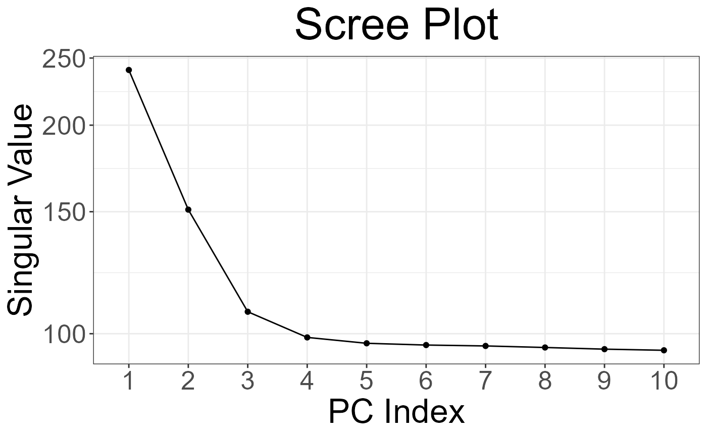
Relative size of text. Default is 1.

viridis

Deprecated argument.

cols

Deprecated. Use ncol instead.

...

Not used.

Value

A ggplot2 object. You can plot it using the print method. You can modify it as you wish by adding layers. You might want to read this chapter

to get more familiar with the package ggplot2.

Examples

set.seed(1)

X <- big_attachExtdata()
svd <- big_SVD(X, big_scale(), k = 10)

# screeplots
plot(svd) # 3 PCs seems "significant"

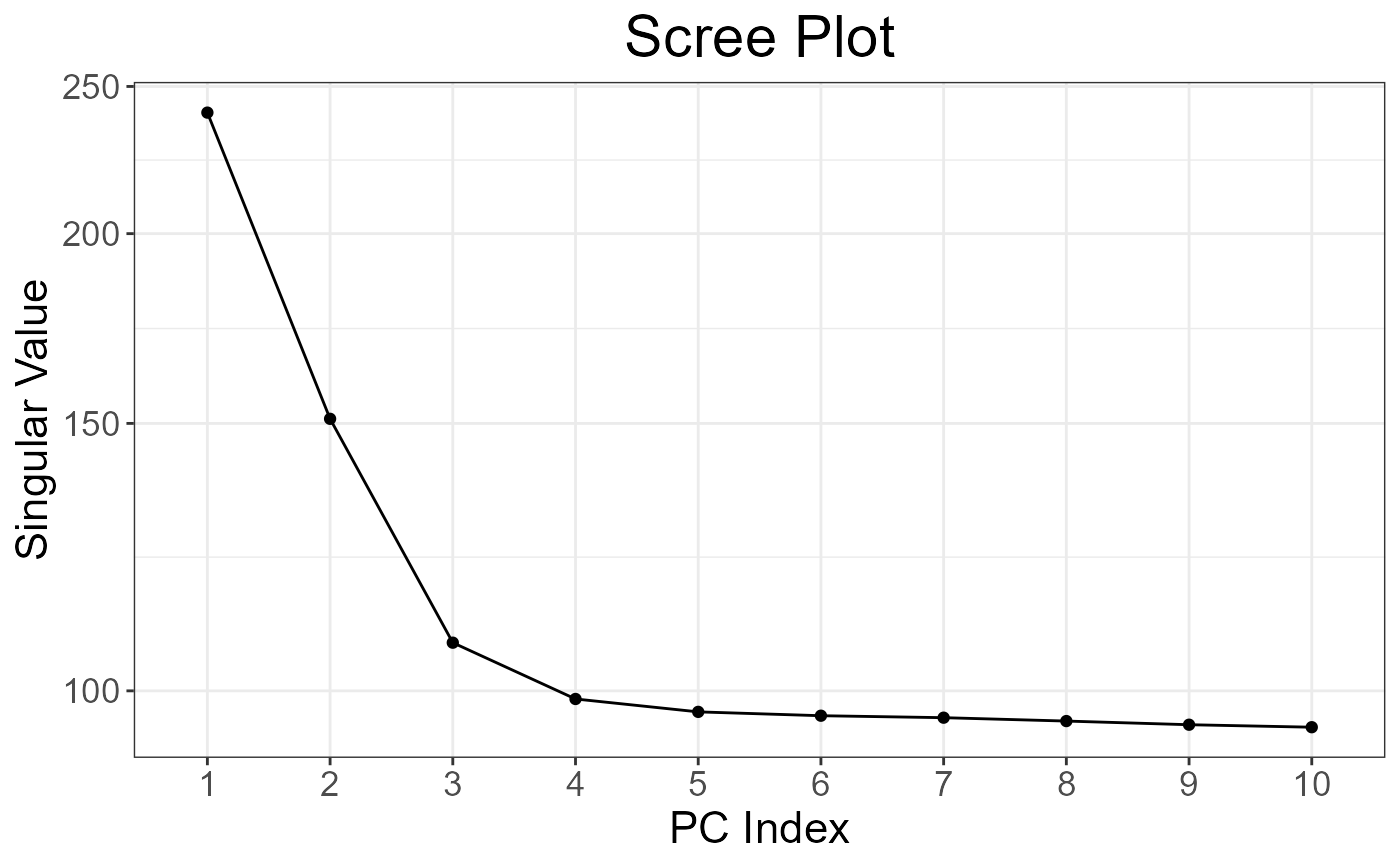plot(svd, coeff = 1.5) # larger font for papers


# scores plot
plot(svd, type = "scores") # first 2 PCs

plot(svd, type = "scores", scores = c(1, 3))

plot(svd, type = "scores", scores = 1:4, ncol = 2, coeff = 0.7)

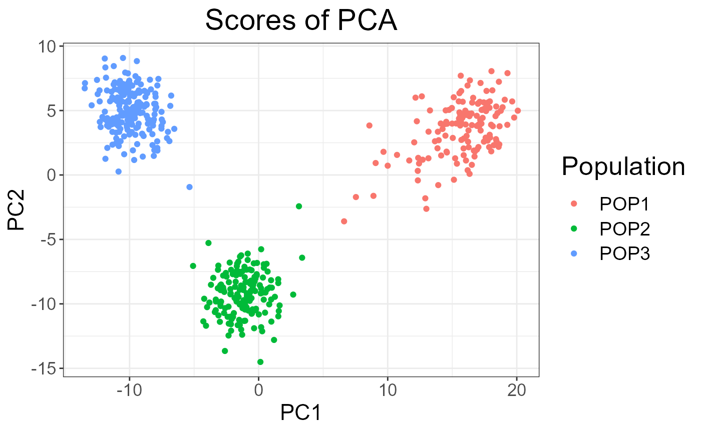
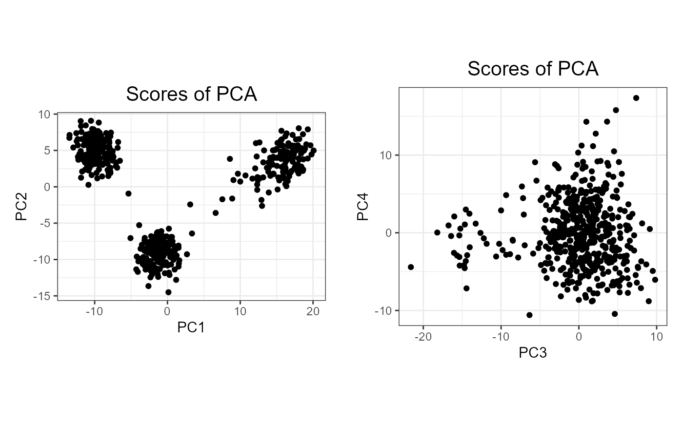## add color (recall that this return a `ggplot2` object)
class(obj <- plot(svd, type = "scores"))
#> [1] "gg"     "ggplot"
pop <- rep(c("POP1", "POP2", "POP3"), c(143, 167, 207))
library(ggplot2)
print(obj2 <- obj + aes(color = pop) + labs(color = "Population"))

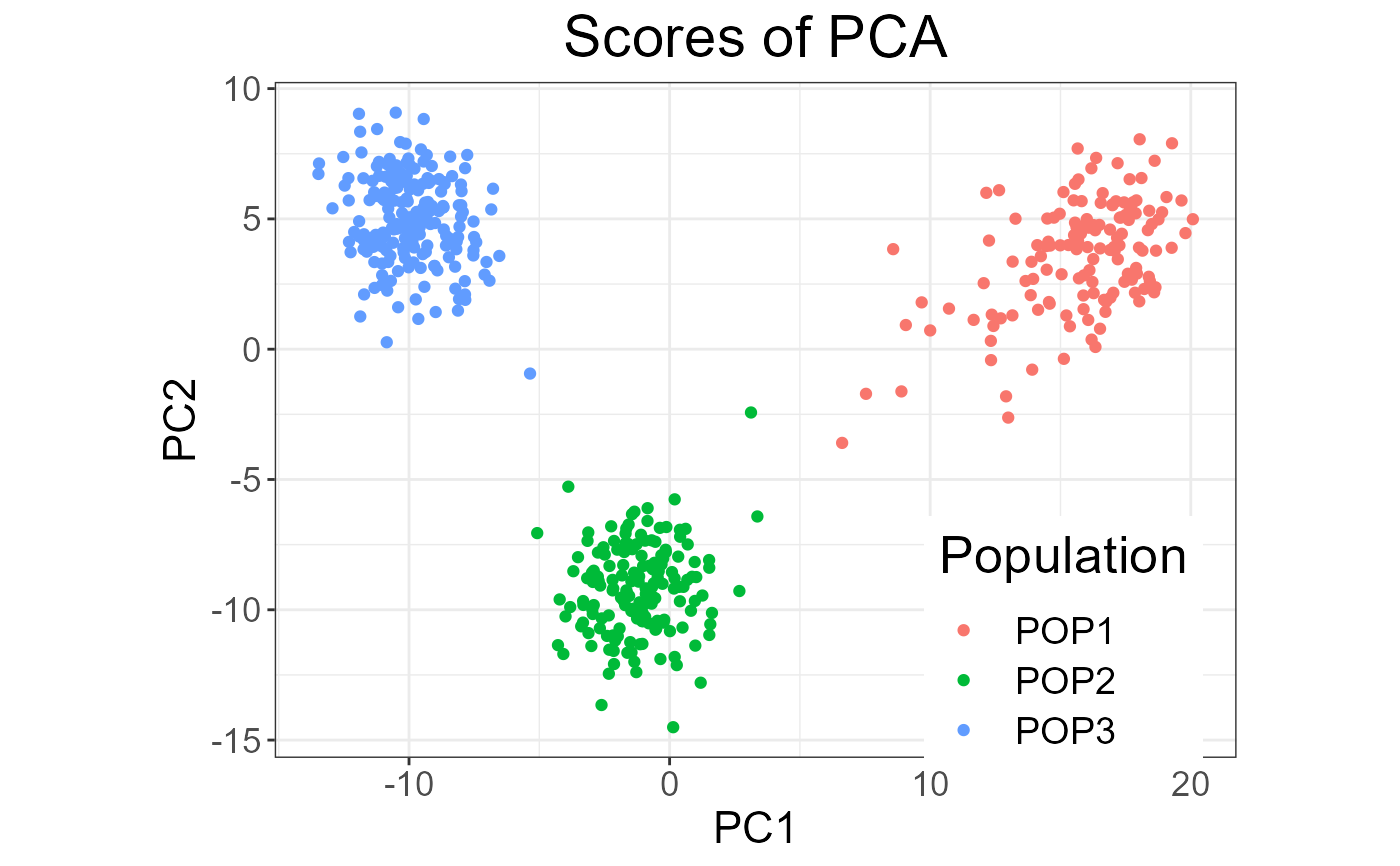
## change the place of the legend
print(obj3 <- obj2 + theme(legend.position = c(0.82, 0.17)))

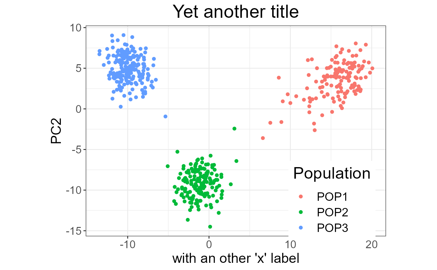
## change the title and the labels of the axes
obj3 + ggtitle("Yet another title") + xlab("with an other 'x' label")


# loadings
plot(svd, type = "loadings", loadings = 2)

## all loadings
plot(svd, type = "loadings", loadings = 1:2, coeff = 0.7, ncol = 1)


# Percentage of variance explained by the PCs
# See https://github.com/privefl/bigstatsr/issues/83

# dynamic plots, require the package **plotly**
if (FALSE) plotly::ggplotly(obj3)

Arguments

Value

See also

Examples