Chapter 5 Genome-Wide Association Study (GWAS)
In bigstatsr, you can perform both standard linear and logistic regressions GWAS, using either big_univLinReg() or big_univLogReg().
Function big_univLinReg() should be very fast, while big_univLogReg() is slower.
This type of association, where each variable is considered independently, can be performed for any type of FBM (i.e. it does not have to be a genotype matrix). This is why these two functions are in package bigstatsr, and not bigsnpr.
5.1 Example
Let’s reuse the data prepared in 3.3 and the PCs in 4.4.
#> Loading required package: bigstatsrThe clinical data includes age, sex, high-density lipoprotein (HDL)-cholesterol (hdl), low-density lipoprotein (LDL)-cholesterol (ldl), triglycerides (tg) and coronary artery disease status (CAD).
For the set of covariates, we will use sex, age, and the first 6 PCs:
PCs are used as covariates in GWAS to correct for population structure (Price et al., 2006).
You probably should not account for other information such as cholesterol as they are heritable covariates, which can lead to collider bias (Aschard, Vilhjálmsson, Joshi, Price, & Kraft, 2015; Day, Loh, Scott, Ong, & Perry, 2016).
G <- obj.bigsnp$genotypes
y <- obj.bigsnp$fam$CAD
ind.gwas <- which(!is.na(y) & complete.cases(covar))
To only use a subset of the data stored as an FBM (G here), you should almost never make a copy of the data; instead, use parameters ind.row (or ind.train) and ind.col to apply functions to a subset of the data.
Let’s perform a case-control GWAS for CAD:
gwas <- runonce::save_run(
  big_univLogReg(G, y[ind.gwas], ind.train = ind.gwas,
                 covar.train = covar[ind.gwas, ], ncores = NCORES),
  file = "tmp-data/GWAS_CAD.rds")
#> user system elapsed
#> 0.17 0.14 157.05
#> Code finished running at 2025-06-10 13:44:27 CESTThis takes about two minutes with 4 cores on my laptop. Note that big_univLinReg() takes two seconds only, and should give very similar p-values, if you just need something quick.
CHR <- obj.bigsnp$map$chromosome
POS <- obj.bigsnp$map$physical.pos
snp_manhattan(gwas, CHR, POS, npoints = 50e3) +
ggplot2::geom_hline(yintercept = -log10(5e-8), linetype = 2, color = "red")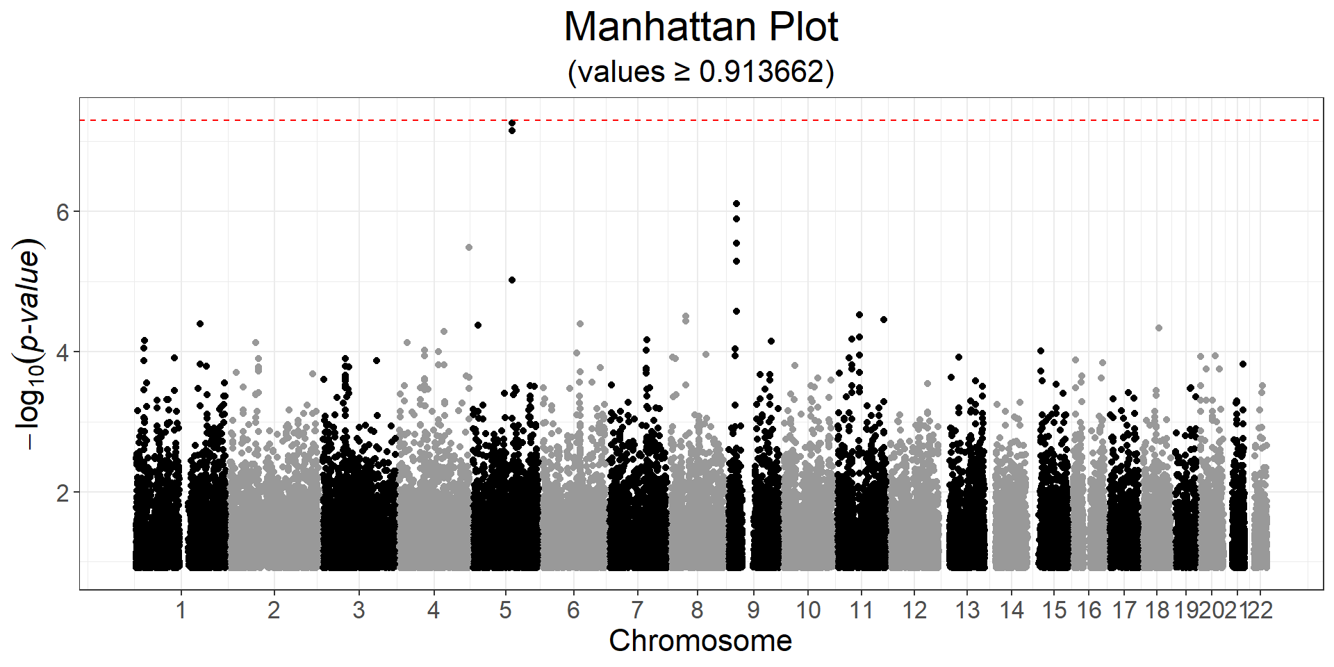 Here, nothing is genome-wide significant because of the small sample size.
Normally, a p-value threshold of \(5 \times 10^{-8}\) is used when reporting significant findings, which corresponds to correcting for one million independent tests. Now, with larger GWAS datasets that include tens of millions of variants, researchers have started using an even more stringent threshold of \(5 \times 10^{-9}\).
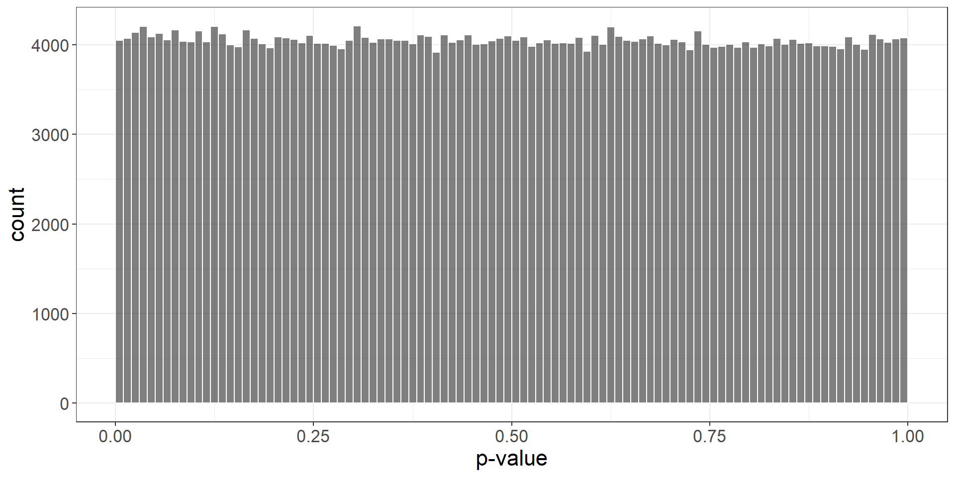
Perform a GWAS for the other phenotypes, and look at the histogram, Q-Q plot and Manhattan plot.
Click to see solution
y2 <- obj.bigsnp$fam$hdl
ind.gwas2 <- which(!is.na(y2) & complete.cases(covar))
gwas2 <- big_univLinReg(G, y2[ind.gwas2], ind.train = ind.gwas2,
                        covar.train = covar[ind.gwas2, ], ncores = NCORES)
snp_manhattan(gwas2, CHR, POS, npoints = 50e3) +
  ggplot2::geom_hline(yintercept = -log10(5e-8), linetype = 2, color = "red")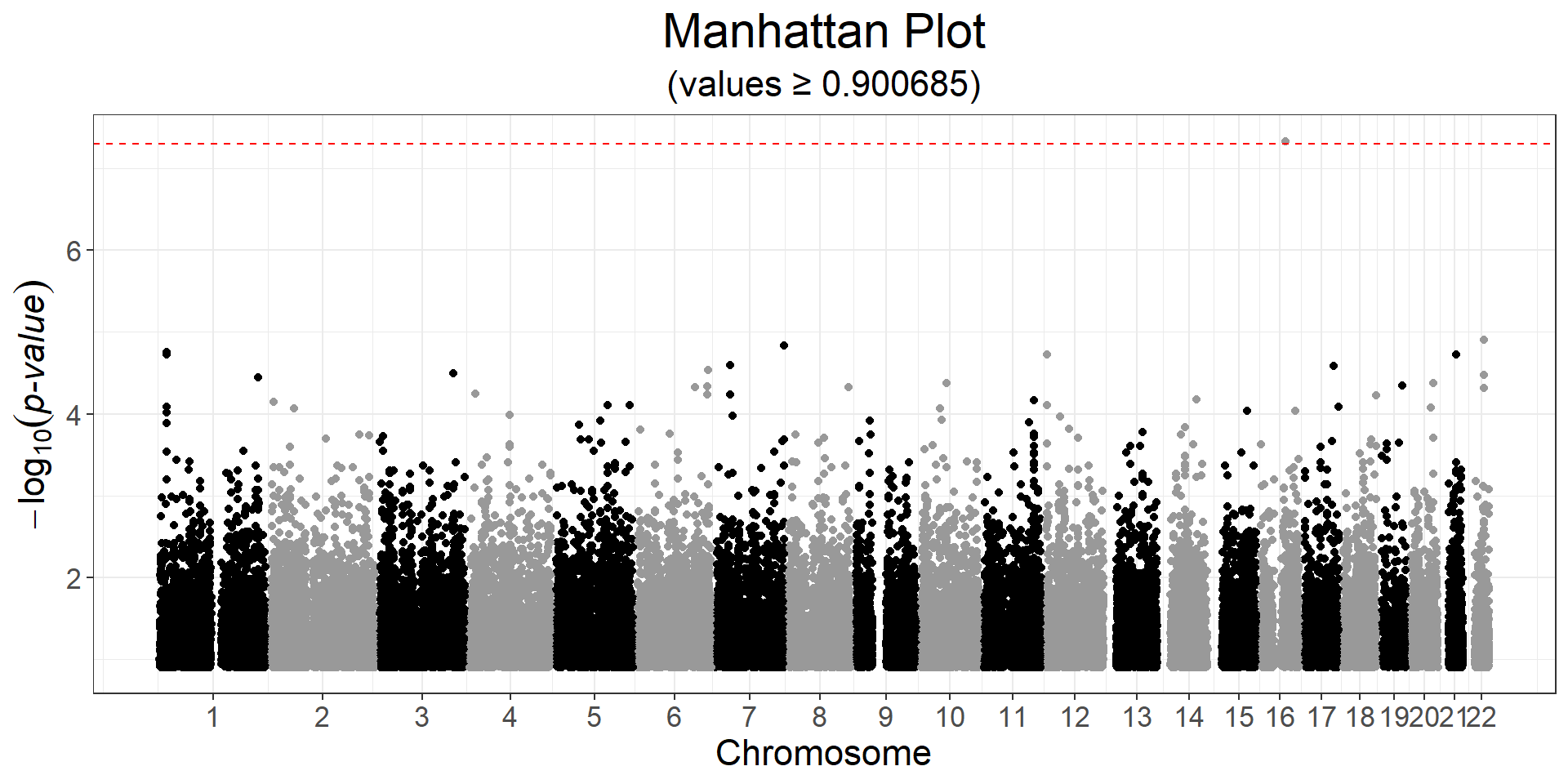
To report independent findings (instead of all variants in one peak), researchers have used LD clumping, which iteratively keeps the most associated variant and remove those that are too correlated with this one. Another strategy is to use GCTA-COJO (Yang et al., 2012).
Perform some LD clumping for all variants with a p-value lower than \(10^{-5}\), using a stringent \(r^2\) threshold of 0.05 over a 5 Mb (= 5000 kb) window. How many variants are left?
Click to see solution
lpval <- -predict(gwas)  # -log10(pval)
ind_keep <- snp_clumping(G, CHR, S = lpval, thr.r2 = 0.05,
                         size = 5000, infos.pos = POS,
                         exclude = which(lpval < -log10(1e-5)),
                         ncores = NCORES)
obj.bigsnp$map[ind_keep, ]
#> chromosome marker.ID genetic.dist physical.pos allele1 allele2
#> 121561 4 rs4863155 0 190300221 G A
#> 136435 5 rs4957723 0 107157011 C T
#> 224210 9 rs9632884 0 22072301 G Csnp_manhattan(gwas, CHR, POS, npoints = 50e3, ind.highlight = ind_keep) +
ggplot2::geom_hline(yintercept = -log10(5e-8), linetype = 2, color = "red") +
ggplot2::geom_hline(yintercept = -log10(1e-5), linetype = 2, color = "blue")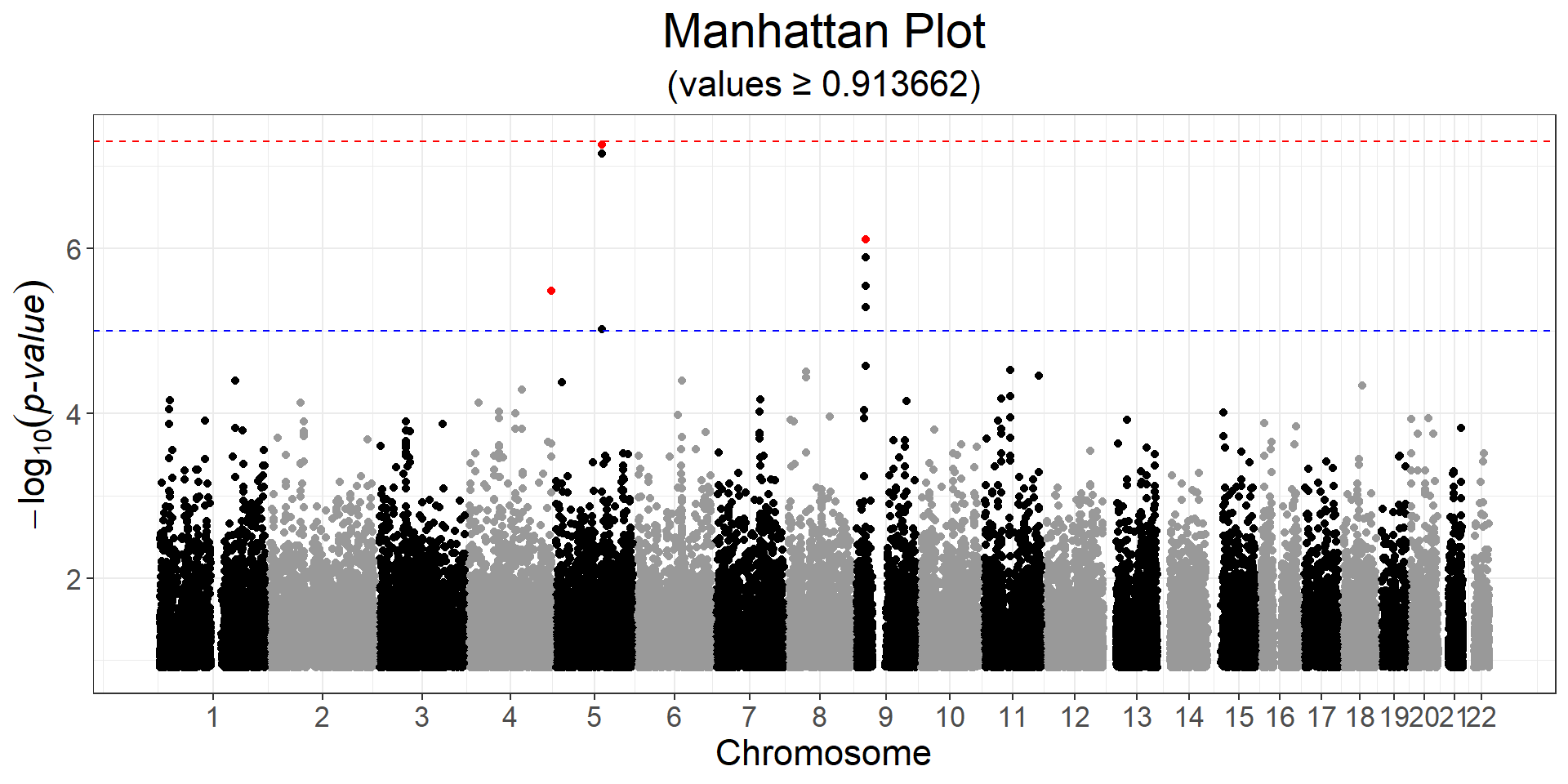
For some example code to run a GWAS on multiple nodes on an HPC cluster:
- GWAS in iPSYCH; you can perform the GWAS on multiple nodes in parallel that would each process a chunk of the variants only
- GWAS for very large data and multiple phenotypes; you should perform the GWAS for all phenotypes for a “small” chunk of columns to avoid repeated access from disk, and can process these chunks on multiple nodes in parallel
- some template for {future.batchtools} when using Slurm
5.2 REGENIE
regenie (Mbatchou et al., 2021) is a C++ program for whole genome regression modeling of large genome-wide association studies. It is developed and supported by a team of scientists at the Regeneron Genetics Center. It is fancier than simple linear/logistic regressions and is currently (one of if not) the state-of-the-art GWAS method.
REGENIE has the following properties:
It supports the BGEN, PLINK bed/bim/fam and PLINK2 pgen/pvar/psam genetic data formats
It works on both quantitative and binary traits, including binary traits with unbalanced case-control ratios
It can handle population structure and relatedness
It can provide some power boost
It is fast and memory efficient 🔥
It can process multiple phenotypes at once efficiently
For binary traits, it supports Firth logistic regression and an SPA test (useful in case of very unbalanced phenotypes)
It can perform gene/region-based tests (burden, SBAT, SKAT/SKATO, ACATV/ACATO)
It can perform interaction tests (GxE, GxG) as well as conditional analyses
Meta-analysis of REGENIE summary statistics can be performed using REMETA
It can be installed with Conda
5.3 Genomic control and LD score regression
\(\lambda_\text{GC}\), the genomic inflation factor (GIF), was used a lot to assess whether a GWAS is confounded by population structure or relatedness (when e.g. larger than 1.05). It corresponds to the ratio between the median of test statistics over the median of expected test statistics (under the null hypothesis). However, it is no longer used because, with sufficient GWAS power and trait polygenicity, a GIF larger than 1 is actually expected (Yang et al., 2011).
#> Warning: Removed 363713 rows containing missing values or values outside the scale range
#> (`geom_point()`).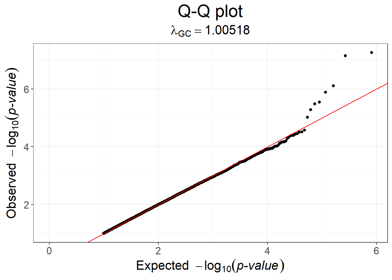
Then, the intercept of LD score regression was introduced to test for confounding (B. K. Bulik-Sullivan et al., 2015). However, note that it was observed that LD score regression intercepts tend to increase with SNP-heritability and GWAS sample size (Loh, Kichaev, Gazal, Schoech, & Price, 2018).
5.4 Some post GWAS analyses
It is challenging to interpret a GWAS on its own as there are often many associations, many of which are in non-coding regions. There is a large collection of downstream analyses to aid in gaining biological understanding from your GWAS, some of which are based on GWAS summary statistics which will cover later in this course.
There are several online tools/resources that allow you to quickly get a sense of the meaning of a variant or GWAS results. If you want to understand what is known about a particular variant, SNPedia, dbSNP, and OpenTargets are good places to start. Here you can find information on the peer-reviewed papers that mention this particular variant, its allele frequencies across populations, its predicted consequences, and associations with other traits.
GTEx is a database of the genetic regulation of gene expression in humans, and is also useful to get a sense of whether a variant of interest may influence the expression of a particular gene. Variants in non-coding regions are generally hypothesized to affect the trait through regulatory mechanisms. This database is not an exhaustive list of genetic regulation of gene expression – a variant may influence gene expression in certain cell or tissue types or contexts not captured in the data.
FUMA is a website where you can upload GWAS summary statistics and it will run a range of analyses to link genetic variants to genes. You can then further investigate these genes with pathways analyses on the same platform. To my knowledge, there is no good tool that can run a range of analyses locally in one go – this would certainly save me a lot of time and be more efficient!
Resources for helping linking GWAS hits to eQTLs:
Read more in this PowerPoint presentation.