Chapter 6 Genome-Wide Association Study (GWAS)

In {bigstatsr}, you can perform both standard linear and logistic regressions GWAS, using either big_univLinReg() or big_univLogReg(). Function big_univLinReg() should be very fast, while big_univLogReg() is slower.

This type of association, where each variable is considered independently, can be performed for any type of FBM (i.e. it does not have to be a genotype matrix). This is why these two functions are in package {bigstatsr}, and not {bigsnpr}.

6.1 Example

Let us reuse the data prepared in 4.3 and the PCs in 5.2.

library(bigsnpr)

#> Loading required package: bigstatsr

obj.bigsnp <- snp_attach("tmp-data/GWAS_data_sorted_QC.rds")

obj.svd <- readRDS("tmp-data/PCA_GWAS_data.rds")
PC <- predict(obj.svd)

The clinical data includes age, sex, high-density lipoprotein (HDL)-cholesterol (hdl), low-density lipoprotein (LDL)-cholesterol (ldl), triglycerides (tg) and coronary artery disease status (CAD).

For the set of covariates, we will use sex, age, and the first 6 PCs:

covar <- cbind(as.matrix(obj.bigsnp$fam[c("sex", "age")]), PC[, 1:6])

You probably should not account for other information such as cholesterol as they are heritable covariates (Aschard, Vilhjálmsson, Joshi, Price, & Kraft, 2015; Day, Loh, Scott, Ong, & Perry, 2016).

G <- obj.bigsnp$genotypes
y <- obj.bigsnp$fam$CAD
ind.gwas <- which(!is.na(y) & complete.cases(covar))

To only use a subset of the data stored as an FBM (G here), you should almost never make a copy of the data; instead, use parameters ind.row (or ind.train) and ind.col to apply functions to a subset of the data.

Let us perform a case-control GWAS for CAD:

gwas <- runonce::save_run(
  big_univLogReg(G, y[ind.gwas], ind.train = ind.gwas,
                 covar.train = covar[ind.gwas, ], ncores = nb_cores()),
  file = "tmp-data/GWAS_CAD.rds")

#>    user  system elapsed 
#>    0.13    0.07  136.54

This takes about two minutes with 4 cores on my laptop. Note that big_univLinReg() takes two seconds only, and should give very similar p-values, if you just need something quick.

plot(gwas)

CHR <- obj.bigsnp$map$chromosome
POS <- obj.bigsnp$map$physical.pos
snp_manhattan(gwas, CHR, POS, npoints = 50e3) +
  ggplot2::geom_hline(yintercept = -log10(5e-8), linetype = 2, color = "red")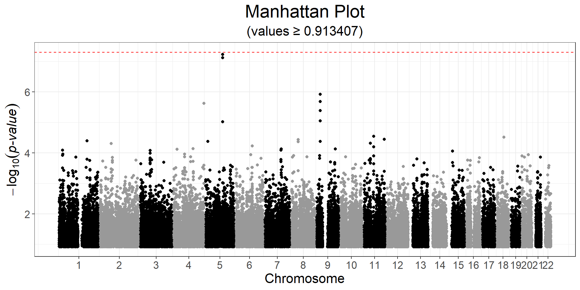

Here, nothing is genome-wide significant because of the small sample size.

y2 <- obj.bigsnp$fam$hdl
ind.gwas2 <- which(!is.na(y2) & complete.cases(covar))
gwas2 <- big_univLinReg(G, y2[ind.gwas2], ind.train = ind.gwas2,
                        covar.train = covar[ind.gwas2, ], ncores = nb_cores())
snp_manhattan(gwas2, CHR, POS, npoints = 50e3) +
  ggplot2::geom_hline(yintercept = -log10(5e-8), linetype = 2, color = "red")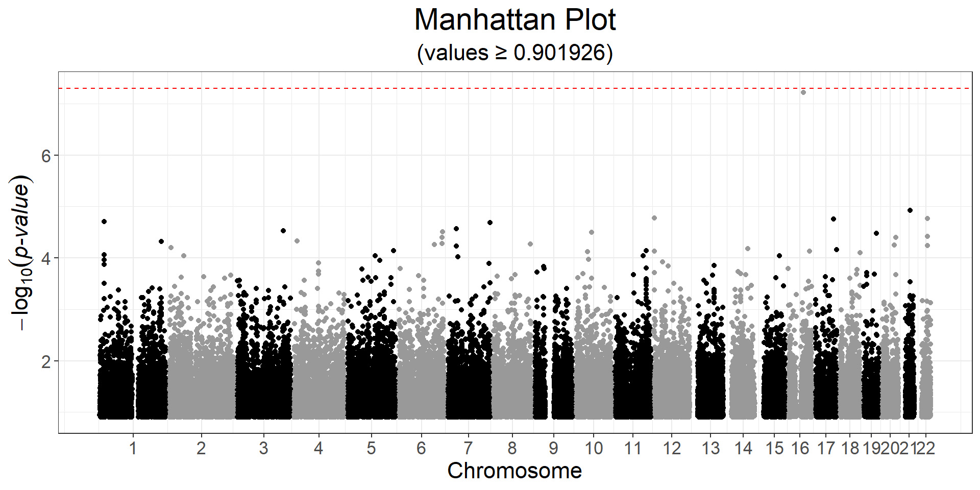

---

Some other example code:

• GWAS in iPSYCH; you can perform the GWAS on multiple nodes in parallel that would each process a chunk of the variants only
• GWAS for very large data and multiple phenotypes; you should perform the GWAS for all phenotypes for a “small” chunk of columns to avoid repeated access from disk, and can process these chunks on multiple nodes in parallel
• some template for {future.batchtools} when using Slurm

References

Aschard, H., Vilhjálmsson, B.J., Joshi, A.D., Price, A.L., & Kraft, P. (2015). Adjusting for heritable covariates can bias effect estimates in genome-wide association studies. The American Journal of Human Genetics, 96, 329–339.

Day, F.R., Loh, P.-R., Scott, R.A., Ong, K.K., & Perry, J.R. (2016). A robust example of collider bias in a genetic association study. The American Journal of Human Genetics, 98, 392–393.