Chapter 7 Polygenic scores (PGS)
Improving PGS methods is the main topic of my research work. These are the main methods currently available in the packages:
efficient penalized regressions, with individual-level data (Privé, Aschard, et al. (2019) + tutorial)
Clumping and Thresholding (C+T) and Stacked C+T (SCT), with summary statistics and individual level data (Privé, Vilhjálmsson, et al. (2019) + tutorial)
LDpred2, with summary statistics (Privé, Arbel, et al. (2020) + tutorial)
lassosum2, with the same input data as LDpred2 (Privé, Arbel, et al. (2022) + tutorial)
7.1 Example: LDpred2 and lassosum2
You should also check the other tutorial mentioned before.
7.1.1 Preparing the data
Let us first read the data produced in 4.3:
#> Loading required package: bigstatsrobj.bigsnp <- snp_attach("tmp-data/GWAS_data_sorted_QC.rds")
G <- obj.bigsnp$genotypes
NCORES <- nb_cores()
map <- dplyr::transmute(obj.bigsnp$map,
chr = chromosome, pos = physical.pos,
a0 = allele2, a1 = allele1)Download some GWAS summary statistics for CAD that I derived from the UK Biobank (Bycroft et al., 2018), and prepare them in the format required by LDpred2:
gz <- runonce::download_file(
  "https://figshare.com/ndownloader/files/38077323",
  dir = "tmp-data", fname = "sumstats_CAD_tuto.csv.gz")
readLines(gz, n = 3)
#> [1] "chr,pos,rsid,allele1,allele2,freq,info,beta,se"
#> [2] "1,721290,rs12565286,C,G,0.035889027911808,0.941918079726998,0.0361758959140647,0.0290865883937757"
#> [3] "1,752566,rs3094315,A,G,0.840799909379283,0.997586884856296,-0.0340838522604864,0.0144572980122262"sumstats <- bigreadr::fread2(
gz,
select = c("chr", "pos", "allele2", "allele1", "beta", "se", "freq", "info"),
col.names = c("chr", "pos", "a0", "a1", "beta", "beta_se", "freq", "info"))
# GWAS effective sample size for binary traits (4 / (1 / n_case + 1 / n_control))
# For quantitative traits, just use the total sample size for `n_eff`.
sumstats$n_eff <- 4 / (1 / 20791 + 1 / 323124) Note that we recommend to use imputed HapMap3+ variants when available, for which you can download some precomputed LD reference for European individuals based on the UK Biobank. Otherwise use the genotyped variants as I am doing here. Try to use an LD reference with at least 2000 individuals (I have only 1401 in this example). Please see this other tutorial for more information.
Let us now match the variants in the GWAS summary statistics with the internal data we have:
library(dplyr)
info_snp <- snp_match(sumstats, map, return_flip_and_rev = TRUE) %>%
  mutate(freq = ifelse(`_REV_`, 1 - freq, freq),
         `_REV_` = NULL, `_FLIP_`= NULL) %>%
  print()
#> chr pos a0 a1 beta beta_se freq info n_eff
#> 1 1 752566 T C 0.034083852 0.01445730 0.15920009 0.9975869 78136.41
#> 2 1 785989 G A 0.018289010 0.01549153 0.13007399 0.9913233 78136.41
#> 3 1 798959 G A 0.003331013 0.01307707 0.20524280 0.9734898 78136.41
#> 4 1 947034 T C -0.021202725 0.02838148 0.03595249 0.9924989 78136.41
#> _NUM_ID_.ss _NUM_ID_
#> 1 2 2
#> 2 4 4
#> 3 5 5
#> 4 6 6
#> [ reached 'max' / getOption("max.print") -- omitted 340206 rows ]Check the summary statistics; some quality control may be needed:
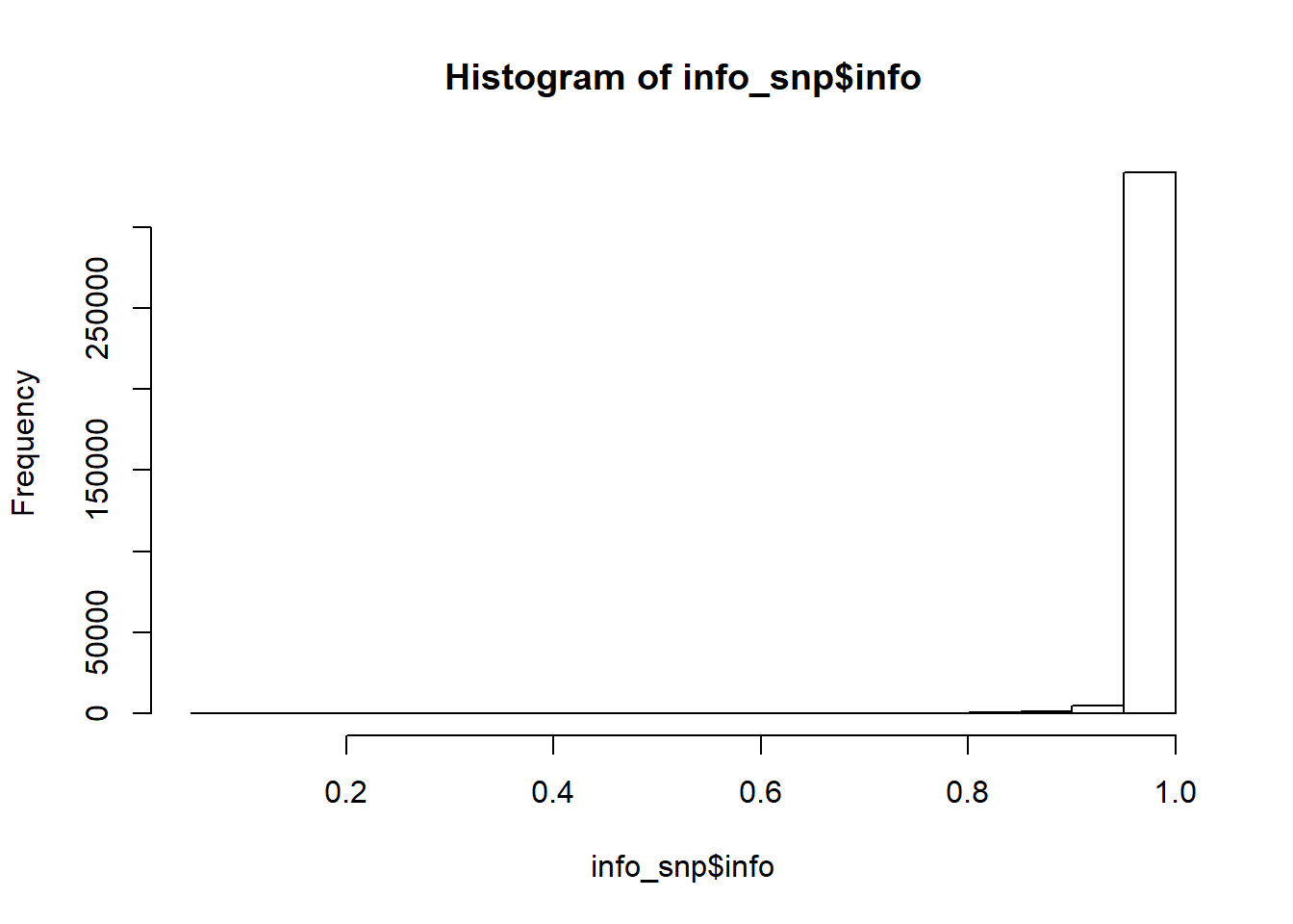
#>      Min.   1st Qu.    Median      Mean   3rd Qu.      Max.
#> 0.0000027 0.1100250 0.2261357 0.2365588 0.3580946 0.9998703
Then we can perform some quality control on the summary statistics by checking whether standard deviations (of genotypes) inferred from the external GWAS summary statistics are consistent with the ones in the internal data we have:
af_ref <- big_colstats(G, ind.col = info_snp$`_NUM_ID_`, ncores = NCORES)$sum / (2 * nrow(G))
sd_ref <- sqrt(2 * af_ref * (1 - af_ref))
sd_ss <- with(info_snp, 2 / sqrt(n_eff * beta_se^2 + beta^2))
is_bad <-
sd_ss < (0.5 * sd_ref) | sd_ss > (sd_ref + 0.1) |
sd_ss < 0.05 | sd_ref < 0.05 # basically filtering small MAF
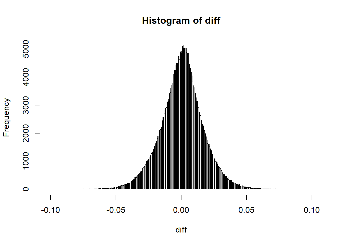
library(ggplot2)#> Warning: package 'ggplot2' was built under R version 4.2.3ggplot(slice_sample(data.frame(sd_ref, sd_ss, is_bad), n = 50e3)) +
geom_point(aes(sd_ref, sd_ss, color = is_bad), alpha = 0.5) +
theme_bigstatsr(0.9) +
scale_color_viridis_d(direction = -1) +
geom_abline(linetype = 2) +
labs(x = "Standard deviations in the reference set",
y = "Standard deviations derived from the summary statistics",
color = "To remove?")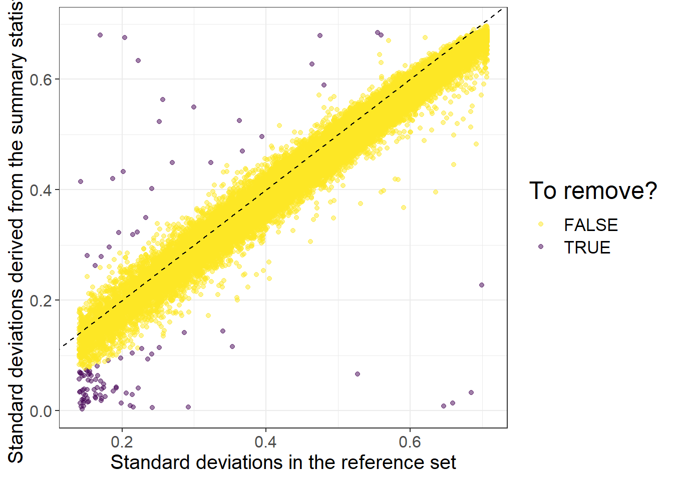
When using quantitative traits (linear regression instead of logistic regression for the GWAS), you need to replace 2 by sd(y) when computing sd_ss (equations 1 and 2 of Privé, Arbel, et al. (2022)).
When allele frequencies are available in the GWAS summary statistics, you can use them (along with INFO scores) to get an even better match:
sd_af <- with(info_snp, sqrt(2 * freq * (1 - freq) * info))
ggplot(slice_sample(data.frame(sd_af, sd_ss), n = 50e3)) +
geom_point(aes(sd_af, sd_ss), alpha = 0.5) +
theme_bigstatsr(0.9) +
geom_abline(linetype = 2, color = "red") +
labs(x = "Standard deviations derived from allele frequencies",
y = "Standard deviations derived from the summary statistics")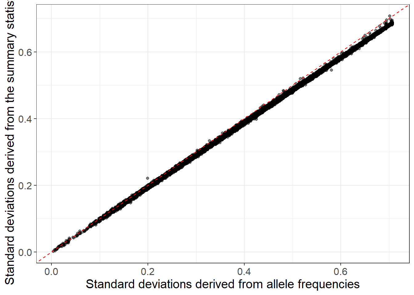 You can still use the reference panel to do some quality control by comparing allele frequencies:
Then you can filter
is_bad2 <-
  sd_ss < (0.7 * sd_af) | sd_ss > (sd_af + 0.1) |
  sd_ss < 0.05 | sd_af < 0.05 |
  info_snp$info < 0.7 | abs(af_diff) > 0.07
mean(is_bad2)
#> [1] 0.002410276Then, we compute the correlation for each chromosome (note that we are using only 4 chromosomes here, for faster running of this tutorial):
# Precomputed genetic positions (in cM) to avoid downloading large files in this tuto
gen_pos <- readRDS(runonce::download_file(
  "https://figshare.com/ndownloader/files/38247288",
  dir = "tmp-data", fname = "gen_pos_tuto.rds"))

df_beta <- dplyr::filter(df_beta, chr %in% 1:4)  # TO REMOVE (for speed here)

for (chr in 1:4) {  # REPLACE BY 1:22

  print(chr)

  corr0 <- runonce::save_run({

    ## indices in 'sumstats'
    ind.chr <- which(df_beta$chr == chr)
    ## indices in 'G'
    ind.chr2 <- df_beta$`_NUM_ID_`[ind.chr]

    # genetic positions (in cM)
    # POS2 <- snp_asGeneticPos(map$chr[ind.chr2], map$pos[ind.chr2], dir = "tmp-data")
    POS2 <- gen_pos[ind.chr2]  # PRECOMPUTED HERE; USE snp_asGeneticPos() IN REAL CODE

    # compute the banded correlation matrix in sparse matrix format
    snp_cor(G, ind.col = ind.chr2, size = 3 / 1000, infos.pos = POS2,
            ncores = NCORES)

  }, file = paste0("tmp-data/corr_chr", chr, ".rds"))

  # transform to SFBM (on-disk format) on the fly
  if (chr == 1) {
    ld <- Matrix::colSums(corr0^2)
    corr <- as_SFBM(corr0, "tmp-data/corr", compact = TRUE)
  } else {
    ld <- c(ld, Matrix::colSums(corr0^2))
    corr$add_columns(corr0, nrow(corr))
  }
}
#> [1] 1
#> user system elapsed
#> 52.86 0.08 14.04
#> [1] 2
#> user system elapsed
#> 55.50 0.10 14.59
#> [1] 3
#> user system elapsed
#> 47.52 0.08 12.39
#> [1] 4
#> user system elapsed
#> 40.46 0.07 10.55#> [1] 0.5756225Note that you will need at least the same memory as this file size (to keep it cached for faster processing) + some other memory for all the results returned. If you do not have enough memory, processing will be very slow (because you would read the data from disk all the time). If using HapMap3 variants, requesting 60 GB should be enough. For this small example, 8 GB of RAM on a laptop should be enough.
7.1.2 LDpred2
We can now run LD score regression:
(ldsc <- with(df_beta, snp_ldsc(ld, length(ld), chi2 = (beta / beta_se)^2,
                                 sample_size = n_eff, blocks = NULL)))
#> int h2
#> 0.9795999 0.0528327We can now run LDpred2-inf very easily:
# LDpred2-inf
beta_inf <- snp_ldpred2_inf(corr, df_beta, ldsc_h2_est)
pred_inf <- big_prodVec(G, beta_inf, ind.col = df_beta$`_NUM_ID_`)
AUCBoot(pred_inf, obj.bigsnp$fam$CAD)
#> Mean 2.5% 97.5% Sd
#> 0.55135634 0.51913716 0.58247163 0.01629319For LDpred2(-grid), this is the grid we recommend to use:
#> [1] 0.0158 0.0370 0.0528 0.0740#> [1] 1.0e-05 1.8e-05 3.2e-05 5.6e-05 1.0e-04 1.8e-04 3.2e-04 5.6e-04
#> [9] 1.0e-03 1.8e-03 3.2e-03 5.6e-03 1.0e-02 1.8e-02 3.2e-02 5.6e-02
#> [17] 1.0e-01 1.8e-01 3.2e-01 5.6e-01 1.0e+00#> [1] 168 3Here, we will be using this smaller grid instead (for speed in this tutorial):
# smaller grid for tutorial only (USE PREVIOUS ONE IN REAL CODE)
(params <- expand.grid(p = signif(seq_log(1e-4, 0.5, length.out = 16), 2),
                       h2 = round(ldsc_h2_est, 4), sparse = TRUE))
#> p h2 sparse
#> 1 0.00010 0.0528 TRUE
#> 2 0.00018 0.0528 TRUE
#> 3 0.00031 0.0528 TRUE
#> 4 0.00055 0.0528 TRUE
#> 5 0.00097 0.0528 TRUE
#> 6 0.00170 0.0528 TRUE
#> 7 0.00300 0.0528 TRUE
#> 8 0.00530 0.0528 TRUE
#> 9 0.00940 0.0528 TRUE
#> 10 0.01700 0.0528 TRUE
#> 11 0.02900 0.0528 TRUE
#> 12 0.05200 0.0528 TRUE
#> 13 0.09100 0.0528 TRUE
#> 14 0.16000 0.0528 TRUE
#> 15 0.28000 0.0528 TRUE
#> 16 0.50000 0.0528 TRUEbeta_grid <- snp_ldpred2_grid(corr, df_beta, params, ncores = NCORES)
params$sparsity <- colMeans(beta_grid == 0)Then, we can compute the corresponding PGS for all these models, and visualize their performance:
pred_grid <- big_prodMat(G, beta_grid, ind.col = df_beta[["_NUM_ID_"]],
                         ncores = NCORES)

params$score <- apply(pred_grid, 2, function(.x) {
  if (all(is.na(.x))) return(NA)  # models that diverged substantially
  summary(glm(  # simply use `lm()` for quantitative traits
    CAD ~ .x + sex + age, data = obj.bigsnp$fam, family = "binomial"
  ))$coef[".x", 3]
})

ggplot(params, aes(x = p, y = score, color = as.factor(h2))) +
  theme_bigstatsr() +
  geom_point() +
  geom_line() +
  scale_x_log10(breaks = 10^(-5:0), minor_breaks = params$p) +
  facet_wrap(~ sparse, labeller = label_both) +
  labs(y = "GLM Z-Score", color = "h2") +
  theme(legend.position = "top", panel.spacing = unit(1, "lines"))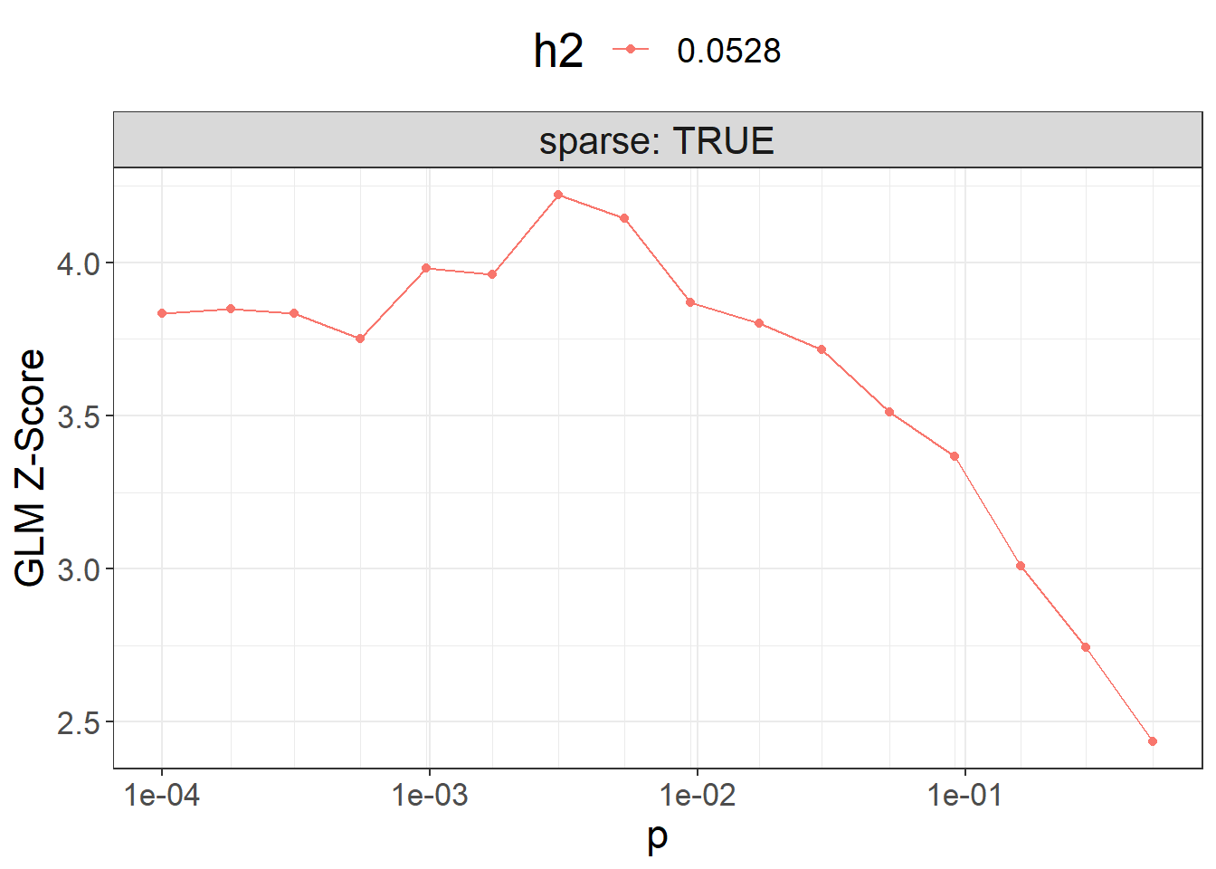
Then you can use the best-performing model here.
Note that, in practice, you should use only individuals from the validation set to compute the $score and then evaluate the best model for the individuals in the test set (unrelated to those in the validation set).
library(dplyr)
best_beta_grid <- params %>%
  mutate(id = row_number()) %>%
  arrange(desc(score)) %>%
  print() %>%
  slice(1) %>%
  pull(id) %>%
  beta_grid[, .]
#> p h2 sparse sparsity score id
#> 1 0.00530 0.0528 TRUE 0.6836137 4.146631 8
#> 2 0.00300 0.0528 TRUE 0.7658781 4.143388 7
#> 3 0.00170 0.0528 TRUE 0.8330722 4.024683 6
#> 4 0.00031 0.0528 TRUE 0.9390631 3.931183 3
#> 5 0.00940 0.0528 TRUE 0.5926931 3.883362 9
#> 6 0.00097 0.0528 TRUE 0.8802609 3.882095 5
#> 7 0.00055 0.0528 TRUE 0.9141125 3.880169 4
#> 8 0.01700 0.0528 TRUE 0.5077554 3.827673 10
#> [ reached 'max' / getOption("max.print") -- omitted 8 rows ]To run LDpred2-auto, you can use:
# LDpred2-auto
multi_auto <- snp_ldpred2_auto(
  corr, df_beta, h2_init = ldsc_h2_est,
  vec_p_init = seq_log(1e-4, 0.2, 30),
  burn_in = 100, num_iter = 100,         # TO REMOVE, for speed here
  allow_jump_sign = FALSE,
  use_MLE = FALSE,         # USE `TRUE` ONLY FOR GWAS WITH LARGE N AND M
  shrink_corr = 0.95,
  ncores = NCORES)
Perform some quality control on the chains:
# `range` should be between 0 and 2
(range <- sapply(multi_auto, function(auto) diff(range(auto$corr_est))))
#> [1] 0.05610116 0.05485296 0.05246964 0.05362731 0.05411493 0.05406085
#> [7] 0.05565820 0.05556862 0.05443418 0.05596064 0.05481213 0.05544055
#> [13] 0.05330767 0.05400312 0.05438586 0.05610538 0.05529910 0.05288243
#> [19] 0.05425194 0.05505035 0.05456609 0.05453399 0.05215457 0.05496076
#> [25] 0.05389907 0.05279059 0.05341267 0.05361184 0.05305573 0.05466622#> [1] 1 2 4 5 6 7 8 9 10 11 12 13 14 15 16 17 19 20 21 22 24 25 27
#> [24] 28 30To get the final effects / predictions, you should only use chains that pass this filtering:
We can finally test the final prediction
final_pred_auto <- big_prodVec(G, final_beta_auto,
                               ind.col = df_beta[["_NUM_ID_"]],
                               ncores = NCORES)
AUCBoot(final_pred_auto, obj.bigsnp$fam$CAD)
#> Mean 2.5% 97.5% Sd
#> 0.56412881 0.53135864 0.59574614 0.016295087.1.3 lassosum2: grid of models
lassosum2 is a re-implementation of the lassosum model (Mak, Porsch, Choi, Zhou, & Sham, 2017) that now uses the exact same input parameters as LDpred2 (corr and df_beta). It can therefore be run next to LDpred2 and the best model can be chosen using the validation set.
Note that parameter ‘s’ from lassosum has been replaced by a new parameter ‘delta’ in lassosum2, in order to better reflect that the lassosum model also uses L2-regularization (therefore, elastic-net regularization).
beta_lassosum2 <- snp_lassosum2(
  corr, df_beta, ncores = NCORES,
  nlambda = 10, maxiter = 50)      # TO REMOVE, for speed here
As with LDpred2-grid, we can compute the corresponding PGS for all these models, and visualize their performance:
pred_grid2 <- big_prodMat(G, beta_lassosum2, ind.col = df_beta[["_NUM_ID_"]],
                          ncores = NCORES)

params2 <- attr(beta_lassosum2, "grid_param")
params2$score <- apply(pred_grid2, 2, function(.x) {
  if (all(is.na(.x))) return(NA)  # models that diverged substantially
  summary(glm(  # simply use `lm()` for quantitative traits
    CAD ~ .x + sex + age, data = obj.bigsnp$fam, family = "binomial"
  ))$coef[".x", 3]
})

ggplot(params2, aes(x = lambda, y = score, color = as.factor(delta))) +
  theme_bigstatsr() +
  geom_point() +
  geom_line() +
  scale_x_log10(breaks = 10^(-5:0)) +
  labs(y = "GLM Z-Score", color = "delta")
#> Warning: Removed 4 rows containing missing values or values outside the scale range
#> (`geom_point()`).#> Warning: Removed 4 rows containing missing values or values outside the scale range
#> (`geom_line()`).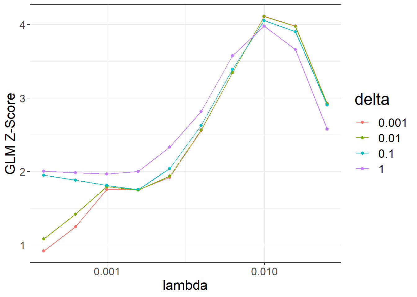
best_grid_lassosum2 <- params2 %>%
  mutate(id = row_number()) %>%
  arrange(desc(score)) %>%
  print() %>%
  slice(1) %>%
  pull(id) %>%
  beta_lassosum2[, .]
#> lambda delta num_iter time sparsity score id
#> 1 0.00996541 0.001 51 0.19 0.9937624 4.112203 3
#> 2 0.00996541 0.010 51 0.18 0.9936938 4.106545 13
#> 3 0.00996541 0.100 45 0.17 0.9930475 4.053764 23
#> 4 0.01579411 0.001 51 0.10 0.9997062 3.977849 2
#> 5 0.00996541 1.000 14 0.05 0.9902959 3.976200 33
#> 6 0.01579411 0.010 51 0.09 0.9997062 3.973049 12
#> 7 0.01579411 0.100 35 0.07 0.9996181 3.900467 22
#> [ reached 'max' / getOption("max.print") -- omitted 33 rows ]We can choose the best-overall model from both LDpred2-grid and lassosum2:
best_grid_overall <- `if`(max(params2$score, na.rm = TRUE) > max(params$score, na.rm = TRUE),
                          best_grid_lassosum2, best_beta_grid)
One advantage of lassosum2 compared to LDpred2 is that it can provide very sparse solutions (< 1% of variants used).