Ancestry proportions and ancestry grouping
Florian Privé
May 11, 2022
Source:vignettes/ancestry.Rmd
ancestry.RmdIn this tutorial, we show how to
estimate ancestry proportions from both summary statistics (allele frequencies) and individual-level data (for each individual whose genotypes are available)
assign individuals into groups of “homogeneous” ancestry
Estimating ancestry proportions from allele frequencies only
This is the primary objective of the method presented in this paper.
For this, let us download some GWAS summary statistics for Epilepsy (supposedly in EUR+EAS+AFR), where the allele frequencies are reported.
DIR <- "../datasets" # you can replace by e.g. "data" or "tmp-data"
# /!\ This downloads 160 Mb
gz <- runonce::download_file(
  "http://www.epigad.org/gwas_ilae2018_16loci/all_epilepsy_METAL.gz",
  dir = "../datasets")
readLines(gz, n = 3)
## [1] "CHR\tBP\tMarkerName\tAllele1\tAllele2\tFreq1\tFreqSE\tWeight\tZscore\tP-value\tDirection\tHetISq\tHetChiSq\tHetDf\tHetPVal"
## [2] "6\t130840091\trs2326918\ta\tg\t0.8470\t0.0178\t36306.88\t-0.279\t0.7805\t-+?\t0.0\t0.117\t1\t0.7321"
## [3] "7\t145771806\trs6977693\tt\tc\t0.8587\t0.0117\t35731.15\t-0.874\t0.3823\t-+?\t0.0\t0.304\t1\t0.5815"
library(dplyr)
sumstats <- bigreadr::fread2(
  gz, select = c("CHR", "BP", "Allele2", "Allele1", "Freq1"),
  col.names = c("chr", "pos", "a0", "a1", "freq")
) %>%
  mutate_at(3:4, toupper)
It is a good idea to filter for the largest per-variant sample sizes (when available..), otherwise this could bias the analyses since ancestry proportions might not be the same for each variant.
Then we need to download the set of reference allele frequencies and corresponding PC loadings (for projection) provided from the paper.
# /!\ This downloads 850 Mb (each)
all_freq <- bigreadr::fread2(
  runonce::download_file("https://figshare.com/ndownloader/files/31620968",
                         dir = DIR, fname = "ref_freqs.csv.gz"))
projection <- bigreadr::fread2(
  runonce::download_file("https://figshare.com/ndownloader/files/31620953",
                         dir = DIR, fname = "projection.csv.gz"))
Then we need to match variants within the summary statistics with the ones from the reference, by chromosome, position and alleles.
## Loading required package: bigstatsr
matched <- snp_match(
  mutate(sumstats, chr = as.integer(chr), beta = 1),
  all_freq[1:5]
) %>%
  mutate(freq = ifelse(beta < 0, 1 - freq, freq))
## 4,880,492 variants to be matched.## 6 ambiguous SNPs have been removed.## 3,343,235 variants have been matched; 0 were flipped and 1,576,097 were reversed.Then we can run the main snp_ancestry_summary()
function. Note that we need to correct for the shrinkage when projecting
a new dataset (here the allele frequencies from the GWAS summary
statistics) onto the PC space.
correction <- c(1, 1, 1, 1.008, 1.021, 1.034, 1.052, 1.074, 1.099,
                1.123, 1.15, 1.195, 1.256, 1.321, 1.382, 1.443)

res <- snp_ancestry_summary(
  freq = matched$freq,
  info_freq_ref = all_freq[matched$`_NUM_ID_`, -(1:5)],
  projection = projection[matched$`_NUM_ID_`, -(1:5)],
  correction = correction
)
The correction factors are needed when projecting
new individuals onto a PCA space to correct for the shrinkage
that happens due to “overfitting” of the PCA. This happens particularly
when the number of individuals used to derive the PCA is smaller than
the number of variables. The amount of correction needed increases for
later PCs. You can have a look at this paper to
read more about this.
Note that the provided correction is specific to the PC
loadings I provide, so that you don’t need to recompute it. It is based
on the ratio between the projections using a method that corrects for
this shrinkage and the simple projections (simply multiplying by the
loadings on the right).
Note that some ancestry groups from the reference are very close to one another, and should be merged a posteriori.
group <- colnames(all_freq)[-(1:5)]
group[group %in% c("Scandinavia", "United Kingdom", "Ireland")]   <- "Europe (North West)"
group[group %in% c("Europe (South East)", "Europe (North East)")] <- "Europe (East)"
grp_fct <- factor(group, unique(group))

final_res <- tapply(res, grp_fct, sum)
round(100 * final_res, 1)
## Africa (West) Africa (South) Africa (East) Africa (North)
## 0.7 0.3 0.0 0.0
## Middle East Ashkenazi Italy Europe (East)
## 0.0 1.8 3.4 13.9
## Finland Europe (North West) Europe (South West) South America
## 6.5 68.0 2.1 0.0
## Sri Lanka Pakistan Bangladesh Asia (East)
## 0.0 0.0 0.0 3.1
## Japan Philippines
## 0.3 0.0Estimating ancestry proportions from individual-level data
This relies on the same principle as in the previous section, but we use genotypes (divided by 2) instead of allele frequencies. We could run the previous function multiple times (i.e. for each individual), but this would be rather slow, so let us “reimplement” it for matrix of genotypes.
Note that this cannot be used for the UK Biobank and the 1000 Genomes data since they are used in the reference, therefore some of these individuals would not need any correction when projecting onto the PC space.
Let us use the Simons Genome Diversity Project (SGDP) data for demonstration.
prefix <- "https://sharehost.hms.harvard.edu/genetics/reich_lab/sgdp/variant_set/cteam_extended.v4.maf0.1perc"
bedfile <- runonce::download_file(paste0(prefix, ".bed"), dir = DIR)
famfile <- runonce::download_file(paste0(prefix, ".fam"), dir = DIR)
bim_zip <- runonce::download_file(paste0(prefix, ".bim.zip"), dir = DIR)
unzip(bim_zip, exdir = DIR, overwrite = FALSE)
## Warning in unzip(bim_zip, exdir = DIR, overwrite = FALSE): not overwriting file
## '../datasets/cteam_extended.v4.maf0.1perc.bimAgain, we need to match the dataset with the reference.
library(bigsnpr)
matched <- sub_bed(bedfile, ".bim") %>%
  bigreadr::fread2(select = c(1, 4:6),
                   col.names = c("chr", "pos", "a1", "a0")) %>%
  mutate(beta = 1) %>%
  snp_match(all_freq[1:5]) %>%
  print()
## 34,418,131 variants to be matched.## 4,365 ambiguous SNPs have been removed.## 4,030,044 variants have been matched; 0 were flipped and 997,183 were reversed.## chr pos a0 a1 beta _NUM_ID_.ss rsid _NUM_ID_
## 1 1 846808 C T 1 3 rs4475691 239
## 2 1 847228 C T 1 13 rs3905286 240
## 3 1 847491 G A 1 17 rs28407778 241
## 4 1 848090 G A 1 24 rs4246505 242
## 5 1 848445 G A 1 35 rs4626817 243
## 6 1 848456 A G 1 36 rs11507767 244
## 7 1 848738 C T 1 46 rs3829741 246
## 8 1 849998 A G -1 75 rs13303222 248
## 9 1 850123 C T 1 79 rs28622257 249
## 10 1 850780 C T -1 86 rs6657440 252
## 11 1 851190 G A 1 94 rs28609852 253
## 12 1 851499 A G -1 102 rs4970465 254
## [ reached 'max' / getOption("max.print") -- omitted 4030032 rows ]Let us read the matched subset of the data and project it onto the PC space.
rds <- snp_readBed2(bedfile, ind.col = matched$`_NUM_ID_.ss`)
obj.bigsnp <- snp_attach(rds)
G <- obj.bigsnp$genotypes
hist(nb_na <- big_counts(G)[4, ])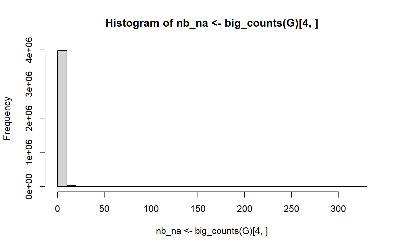
ind <- which(nb_na < 5)        # further subsetting on missing values
G2 <- snp_fastImputeSimple(G)  # imputation when % of missing value is small
# project individuals (divided by 2) onto the PC space
PROJ <- as.matrix(projection[matched$`_NUM_ID_`[ind], -(1:5)])
all_proj <- big_prodMat(G2, sweep(PROJ, 2, correction / 2, '*'),
                        ind.col = ind,
                        # scaling to get G if beta = 1 and (2 - G) if beta = -1
                        center = 1 - matched$beta[ind],
                        scale = matched$beta[ind])
plot(all_proj[, 2:3])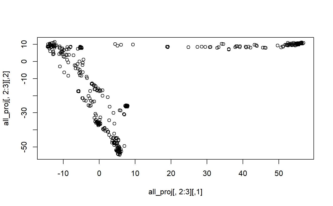
Let us now project the reference allele frequencies, which do not need any correction because these come from the same individuals used to train the PCA.
Now we need to solve a quadratic programming problem for each individual.
cp_X_pd <- Matrix::nearPD(crossprod(X), base.matrix = TRUE)
Amat <- cbind(1, diag(ncol(X)))
bvec <- c(1, rep(0, ncol(X)))

# solve a QP for each projected individual
all_res <- apply(all_proj, 1, function(y) {
  quadprog::solve.QP(
    Dmat = cp_X_pd$mat,
    dvec = crossprod(y, X),
    Amat = Amat,
    bvec = bvec,
    meq  = 1
  )$sol %>%
    tapply(grp_fct, sum) %>%
    round(7)
})
Let us compare the results with the reported information on individuals.
fam2 <- bigreadr::fread2("https://sharehost.hms.harvard.edu/genetics/reich_lab/sgdp/SGDP_metadata.279public.21signedLetter.44Fan.samples.txt")
fam <- dplyr::left_join(obj.bigsnp$fam, fam2, by = c("sample.ID" = "Sample_ID(Aliases)"))
fam_info <- fam[c("Region", "Country", "Population_ID")]

cbind.data.frame(fam_info, round(100 * t(all_res), 1)) %>%
  rmarkdown::paged_table(list(rows.print = 15, max.print = nrow(fam)))
Ancestry grouping
Similar to the previous section, but we want to assign only one label instead of getting ancestry proportions.
We recommend to use Euclidean distance on the PC space for such purposes, as demonstrated in Supp. Note A of this paper. For example, we use this strategy to assign ancestry in the UK Biobank (cf. this code). Normally, admixed individuals or from distant populations should not be matched to any of the 21 reference groups.
PC_SGDP <- all_proj
all_centers <- t(X)
all_sq_dist <- apply(all_centers, 1, function(one_center) {
  rowSums(sweep(PC_SGDP, 2, one_center, '-')^2)
})

thr_fst <- 0.005  # you can adjust this threshold
thr_sq_dist <- max(dist(all_centers)^2) * thr_fst / 0.16

cluster <- group[
  apply(all_sq_dist, 1, function(x) {
    ind <- which.min(x)
    if (isTRUE(x[ind] < thr_sq_dist)) ind else NA
  })
]

table(cluster, exclude = NULL)
## cluster
## Africa (East) Africa (North) Africa (South) Africa (West)
## 11 6 32 23
## Asia (East) Bangladesh Europe (East) Europe (North West)
## 32 3 10 9
## Europe (South West) Finland Italy Japan
## 8 5 8 17
## Middle East Pakistan Philippines South America
## 32 17 8 1
## Sri Lanka <NA>
## 18 105
cbind.data.frame(fam_info, Assigned_group = cluster) %>%
  rmarkdown::paged_table(list(rows.print = 15, max.print = nrow(fam)))
Using this strategy, we can cluster 240 out of 345 individuals. However, we have some trouble clustering Papuans, people from Central Asia and Siberia, people from some African regions, as well as people from South America.
For individuals from South America, we can use the previous ancestry proportions.
cluster[all_res["South America", ] > 0.9] <- "South America"

table(cluster, exclude = NULL)
## cluster
## Africa (East) Africa (North) Africa (South) Africa (West)
## 11 6 32 23
## Asia (East) Bangladesh Europe (East) Europe (North West)
## 32 3 10 9
## Europe (South West) Finland Italy Japan
## 8 5 8 17
## Middle East Pakistan Philippines South America
## 32 17 8 25
## Sri Lanka <NA>
## 18 81
cbind.data.frame(fam_info, Assigned_group = cluster) %>%
  rmarkdown::paged_table(list(rows.print = 15, max.print = nrow(fam)))
References
Privé, Florian. “Using the UK Biobank as a global reference of worldwide populations: application to measuring ancestry diversity from GWAS summary statistics.” Bioinformatics 38.13 (2022): 3477-3480.
Privé, Florian, et al. “Portability of 245 polygenic scores when derived from the UK Biobank and applied to 9 ancestry groups from the same cohort.” The American Journal of Human Genetics 109.1 (2022): 12-23.