PRS

Polygenic Risk Scores with possible clumping and thresholding.

snp_PRS(
  G,
  betas.keep,
  ind.test = rows_along(G),
  ind.keep = cols_along(G),
  same.keep = rep(TRUE, length(ind.keep)),
  lpS.keep = NULL,
  thr.list = 0
)

Arguments

G

A FBM.code256 (typically <bigSNP>$genotypes).
You shouldn't have missing values. Also, remember to do quality control, e.g. some algorithms in this package won't work if you use SNPs with 0 MAF.

betas.keep

Numeric vector of weights associated with each SNP corresponding to ind.keep. You may want to see bigstatsr::big_univLinReg or bigstatsr::big_univLogReg.

ind.test

The individuals on whom to project the scores. Default uses all.

ind.keep

Column (SNP) indices to use (if using clumping, the output of snp_clumping). Default doesn't clump.

same.keep

A logical vector associated with betas.keep whether the reference allele is the same for G. Default is all TRUE (for example when you train the betas on the same dataset). Otherwise, use same_ref.

lpS.keep

Numeric vector of -log10(p-value) associated with betas.keep. Default doesn't use thresholding.

thr.list

Threshold vector on lpS.keep at which SNPs are excluded if they are not significant enough. Default doesn't use thresholding.

Value

A matrix of scores, where rows correspond to ind.test and columns correspond to thr.list.

Examples

test <- snp_attachExtdata()
G <- big_copy(test$genotypes, ind.col = 1:1000)
CHR <- test$map$chromosome[1:1000]
POS <- test$map$physical.position[1:1000]
y01 <- test$fam$affection - 1

# PCA -> covariables
obj.svd <- snp_autoSVD(G, infos.chr = CHR, infos.pos = POS)
#> Discarding 0 variant with MAC < 10 or MAF < 0.02.
#> 
#> Phase of clumping (on MAF) at r^2 > 0.2.. keep 952 variants.
#> 
#> Iteration 1:
#> Computing SVD..
#> 26 outlier variants detected..
#> 
#> Iteration 2:
#> Computing SVD..
#> 0 outlier variant detected..
#> 
#> Converged!

# train and test set
ind.train <- sort(sample(nrow(G), 400))
ind.test <- setdiff(rows_along(G), ind.train) # 117

# GWAS
gwas.train <- big_univLogReg(G, y01.train = y01[ind.train],
                             ind.train = ind.train,
                             covar.train = obj.svd$u[ind.train, ])
# clumping
ind.keep <- snp_clumping(G, infos.chr = CHR,
                         ind.row = ind.train,
                         S = abs(gwas.train$score))
# -log10(p-values) and thresolding
summary(lpS.keep <- -predict(gwas.train)[ind.keep])
#>     Min.  1st Qu.   Median     Mean  3rd Qu.     Max. 
#> 0.000058 0.127537 0.339442 0.470071 0.663226 6.312297 
thrs <- seq(0, 4, by = 0.5)
nb.pred <- sapply(thrs, function(thr) sum(lpS.keep > thr))

# PRS
prs <- snp_PRS(G, betas.keep = gwas.train$estim[ind.keep],
               ind.test = ind.test,
               ind.keep = ind.keep,
               lpS.keep = lpS.keep,
               thr.list = thrs)

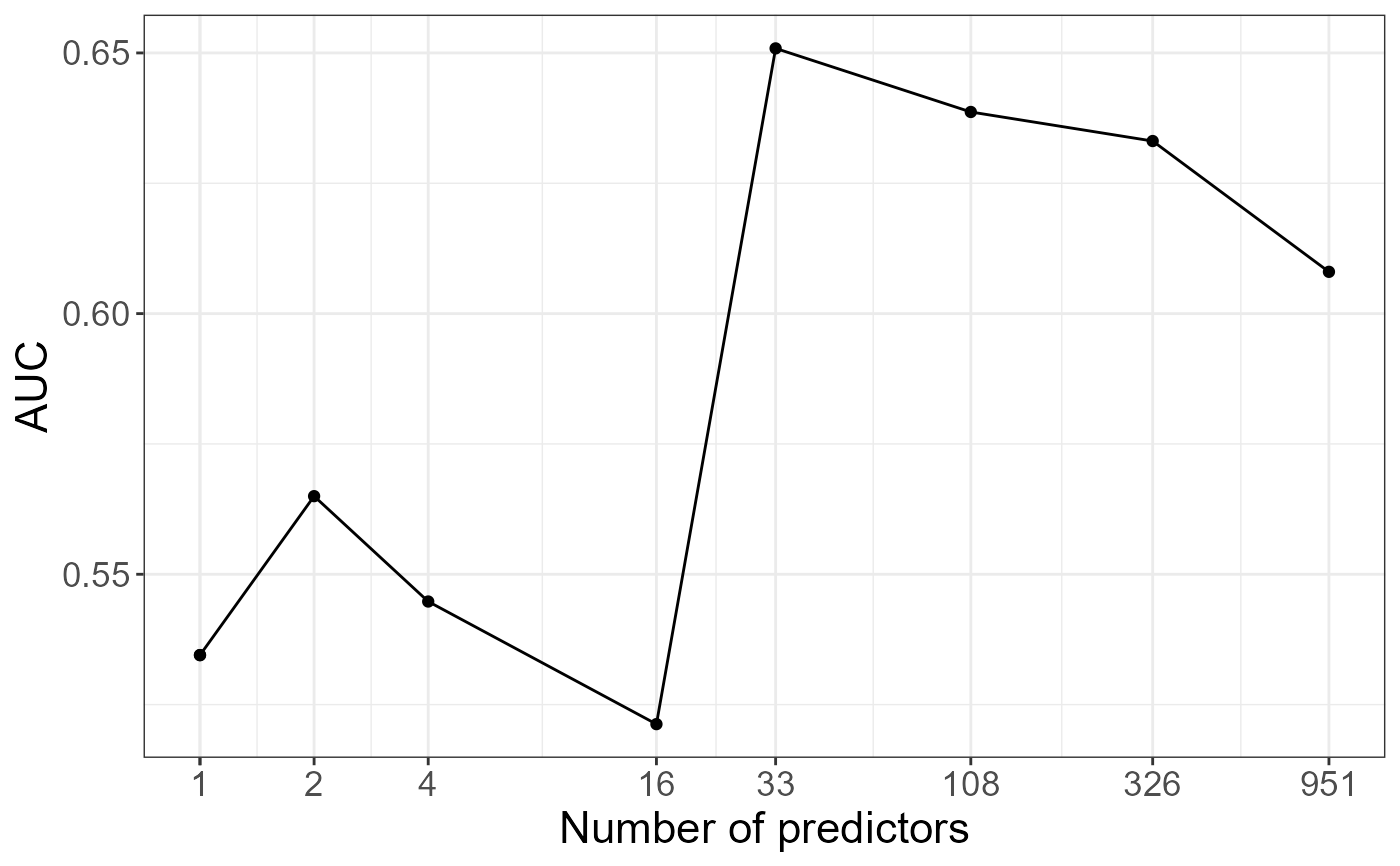
# AUC as a function of the number of predictors
aucs <- apply(prs, 2, AUC, target = y01[ind.test])
library(ggplot2)
#> Warning: package 'ggplot2' was built under R version 4.2.3
qplot(nb.pred, aucs) +
  geom_line() +
  scale_x_log10(breaks = nb.pred) +
  labs(x = "Number of predictors", y = "AUC") +
  theme_bigstatsr()
#> Warning: `qplot()` was deprecated in ggplot2 3.4.0.